Cauchy's inequality: why the square always wins
The AM-GM inequality explains why a square fence encloses the most land, why +50% then −50% leaves you short, and the life of Augustin-Louis Cauchy.

Mục lục
Forty metres of fencing
You have forty metres of fencing and want to enclose a rectangular garden. Fence it 18 by 2 metres and you get 36 square metres. Fence it 15 by 5 and you get 75. Fence a square, 10 by 10, and you get 100 square metres. No rectangle does better.
Why does the square always win? The answer is one line that every Vietnamese student meets at school as Cauchy’s inequality: for two positive numbers and , the arithmetic mean is never smaller than the geometric mean,
and the two sides are equal only when . In English it is usually called the AM-GM inequality (arithmetic mean – geometric mean). For the garden, half the perimeter is always 20 metres, so , the area can never exceed , and it reaches that value only when the two sides are equal: a square.
The inequality carries the name of Augustin-Louis Cauchy, a French mathematician born in 1789, who rebuilt the foundations of calculus and has more concepts named after him than any other mathematician. He did not invent it from scratch, but he proved it for any number of terms, with an argument that textbooks still teach two hundred years later.
This is an episode in the series on mathematicians: the story of an inequality that is all around us, of Cauchy’s life and work, and of a second inequality, also his, that Vietnamese students know under someone else’s name.
Two ways to average
The arithmetic mean is the familiar one: add up and divide. The geometric mean is less familiar, but it is the right answer to every question about growth. When a quantity is multiplied stage by stage, what you need to know is: which steady rate, repeated the same number of times, gives exactly the final result? That rate is the geometric mean.
A product’s price goes up 50%, then down 50% the next month. The arithmetic mean of “+50%” and “−50%” is 0%, which sounds like the price is back where it started. But 150, and 75**. The geometric mean of the two factors 1.5 and 0.5 is : on average, the price actually fell about 13% a month. Cauchy’s inequality says this is no accident: the geometric mean of the factors is always below their arithmetic mean, unless all the factors are equal.
A longer test. A new app launches, and each month its user count either grows 30% or shrinks 20%, exactly twelve months of each over two years. The “average” change is +5% a month, which promises 3.23 times the starting users after 24 months. In reality, whatever order the months come in, the result is always 1.60 times. The real growth rate is the geometric mean , about +2% a month.
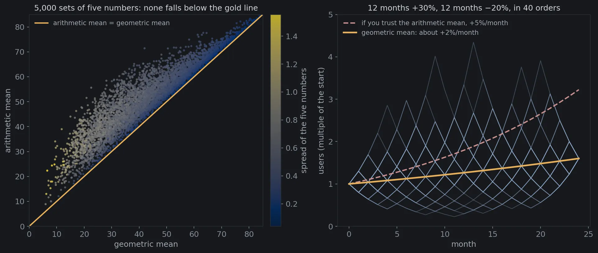
Figure 1 shows one more thing: the further apart the numbers, the further the geometric mean falls behind. For sets of five numbers that are close together, it is less than 1% below the arithmetic mean. For sets that are far apart, it is about a third lower. The stronger the swings, the more the “average on paper” misleads.
One more kind of average
You drive to your hometown at 60 km/h and come back at 40 km/h. What is your average speed for the whole trip? The natural answer is 50 km/h, and it is wrong. If the distance is 120 km, the trip out takes 2 hours and the trip back 3 hours: 240 km in 5 hours, or 48 km/h.
The number 48 is the harmonic mean of 60 and 40. It is always less than or equal to the geometric mean (), which in turn is less than or equal to the arithmetic mean (50). The three averages always line up in that order, and the whole chain also follows from Cauchy’s inequality. Next time someone takes the “average” of speeds, ratios or growth rates, ask: which average?
A proof in one picture
For two numbers, Cauchy’s inequality can be proved with almost no calculation.
Take four identical rectangles with sides and . Arrange them around a centre like the four blades of a pinwheel, forming a large square with side . A small square hole with side is left in the middle. The area of the large square equals the four rectangles plus the hole, and the hole can never have negative area, so
Divide by 4 and take the square root, and you have Cauchy’s inequality. The hole disappears only when , when the four rectangles become four squares that fit perfectly. The equality case, and the square garden, appear right in the picture.
The two-number case is already implicit in Euclid’s Elements. What Cauchy did, as we will see near the end, was prove it for any number of terms. But first, who was Cauchy?
A child of 1789
Augustin-Louis Cauchy was born in Paris on 21 August 1789, a little over a month after the storming of the Bastille. A few years later, as the Terror spread through Paris, the family left for the village of Arcueil on the outskirts to stay safe[1]. Those were lean years: Cauchy later recalled that the family “never had more than half a pound of bread”.
Arcueil was also where his luck began. Pierre-Simon Laplace was a neighbour, and once the family was back in Paris, both Laplace and Joseph-Louis Lagrange visited the house. Lagrange soon saw that the boy was gifted, but his advice was surprising: let him get a solid grounding in languages first, and only then go deep into mathematics[1]. The family followed it. Cauchy studied Greek and Latin, began serious mathematics only in 1804, and in 1805 came second in the entrance examination of the École Polytechnique, France’s most prestigious engineering school.
The engineer who rose at four
In 1810, the 21-year-old engineer was posted to the port of Cherbourg, where Napoleon was building harbour works for the fleet he hoped would invade England. In his luggage were Laplace’s Mécanique céleste and Lagrange’s Théorie des fonctions.
He wrote home: “I get up at four o’clock each morning and I am busy from then on”, adding that the work did not tire him but gave him energy[1]. On the building site, he kept doing mathematics. In 1811 he proved that the angles of a convex polyhedron are completely determined by its faces, a problem Legendre had posed. The result made a strong impression in Paris, and mathematicians began urging the young engineer to devote his life to mathematics. In 1812 he fell ill, possibly partly from exhaustion and depression[1], returned to Paris and never went back to Cherbourg.
The Paris years
In 1816 he won the Grand Prix of the French Academy of Sciences for his work on waves on the surface of water. He was also the first to prove a claim Fermat had left behind in the 17th century: every positive integer is a sum of at most three triangular numbers, at most four squares, at most five pentagonal numbers, and so on[5].
Also in 1816, when the Bourbons returned to the throne, the scientists Gaspard Monge and Lazare Carnot were removed from the Academy for political reasons, and the king appointed Cauchy, then 27, to a vacant seat. Many colleagues found this hard to accept, and his relations with the Paris scientific world were never entirely smooth.
Cours d’analyse: teaching Europe rigour
In 1821, Cauchy published the Cours d’analyse for students at the École Polytechnique[3].
The calculus of Newton and Leibniz was extremely effective at the time, but its foundations were murky. People used “infinitely small” quantities, smaller than any positive number yet not zero, that nobody could explain. Cauchy put the concept of the limit at the centre and carefully defined what it means for a function to be continuous and for an infinite series to converge. The historian Judith Grabiner called him “the man who taught rigorous analysis to all of Europe”[5]. Not every definition of his is perfect by today’s standards, and later generations such as Weierstrass would sharpen them. But the “prove first, then believe” approach of today’s university courses starts with this book.
In the notes at the end of the book, Cauchy placed two inequalities: the arithmetic–geometric mean inequality for numbers, and an inequality about sums of products.
The second inequality: Cauchy’s name, Bunyakovsky’s name
For two sequences of real numbers and ,
with equality when the two sequences are proportional.
Cauchy published the version for sums in 1821. In 1859 the Russian mathematician Viktor Bunyakovsky published the analogous version for integrals, and in 1888 the German mathematician Hermann Schwarz gave the modern proof of the integral version[7]. In English it is the Cauchy–Schwarz inequality. Following the Russian textbook tradition, Vietnamese textbooks name it after Bunyakovsky and reserve Cauchy’s name for the inequality at the start of this article. In fact, both are in the same book by Cauchy.
It has a simple geometric meaning. Think of each sequence as an arrow (a vector) in a space of many dimensions. The inequality says that the dot product of two arrows never exceeds the product of their lengths, so the ratio between them always lies between −1 and 1. That ratio is the cosine of the angle between the arrows. Thanks to it, we can talk about the “angle” between two lists of thousands of numbers, in a space nobody can draw.
And that idea runs in many familiar things:
- Image search and recommendation systems. Every photo, song or user is turned into a list of hundreds of numbers. Two things are “similar” when the cosine of the angle between them is close to 1, a measure called cosine similarity. More in the articles on image search and how YouTube and TikTok recommend videos.
- The correlation coefficient always lies between −1 and 1, because it is the cosine of the angle between two data series shifted to their means. The article on regression to the mean (article in Vietnamese) shows the surprising conclusions this number leads to.
- Heisenberg’s uncertainty principle has a standard proof whose key step is the Cauchy–Schwarz inequality.
Two forgotten manuscripts
Cauchy was a devout Catholic and a loyal supporter of the Bourbon kings. Biographies record that he argued fiercely and that his relations with many colleagues were strained[1]. In the history of mathematics, his name is also tied to the fate of two young mathematicians’ manuscripts.
In 1826, the young Norwegian Niels Henrik Abel submitted to the Academy the work he considered the most important of his life. Cauchy was asked to review it, set the manuscript aside and forgot it. In a letter home, Abel complained that nothing could be done about Cauchy, even though he was the only one at the time who knew how mathematics should be done. The report on the work was written only at the end of June 1829, nearly three months after Abel passed away at 26[1]. The full story is in Abel and the letter that came too late.
Also in 1829, the 17-year-old student Évariste Galois sent his first results to the Academy through Cauchy. The manuscript was not published. Historians still debate how much Cauchy was to blame; some documents suggest he had planned to present the work. But Galois’s ideas became known to the world only years after he passed away. More in Galois, the night before the duel.
It is worth noting that Cauchy was teaching at three institutions at the time, writing dozens of papers a year and receiving a great many manuscripts to review.
Years of exile
In 1830, the July Revolution overthrew King Charles X. The new regime required every official to swear an oath of allegiance, and Cauchy refused. He lost all his teaching posts and left France[1], first for Turin, then in 1833 for Prague, as science tutor to Charles X’s 13-year-old grandson. By many accounts he was not a successful tutor, as his lessons were far too hard for a boy. Even so, the exiled king made him a baron in thanks, a title Cauchy valued highly[5].
He returned to Paris in 1838 and kept his seat at the Academy, but because he still would not take the oath, he could not teach again until 1848. He never stopped writing. In 1847, in a three-page paper on solving systems of equations for astronomical calculations, he proposed: to find the lowest point of a function, take small steps in the direction of steepest descent[4]. Nearly two centuries later, that method, gradient descent, is how almost every AI model is trained, as told in the article on gradient descent.
He also gave much of his time to charity. During the Great Famine in Ireland in the 1840s, he appealed for help for the Irish people, and he helped found several Catholic educational institutions[5].
Augustin-Louis Cauchy passed away in the early morning of 23 May 1857 at Sceaux, near Paris, at the age of 67. According to his daughter, he remained alert until his last hours[1].
Where is Cauchy today?
Hans Freudenthal remarked that more concepts and theorems are named after Cauchy than after any other mathematician[5]: Cauchy sequences, Cauchy’s integral theorem, the Cauchy–Riemann equations, the Cauchy distribution… His collected works, some eight hundred papers, fill 27 volumes published between 1882 and 1970[1].
- Bridges and tall buildings. He founded the theory of stress in elastic materials. The Cauchy stress tensor is in every structural-analysis program. The engineer from Cherbourg still helps build large structures, just in a different way.
- Real numbers. One rigorous way to define the real numbers, including numbers like and , rests on Cauchy sequences: sequences whose terms get ever closer together. Every time a computer adds decimal digit after digit to close in on a number, it follows that same idea.
- Electrical engineering and signal processing use complex analysis every day, a field Cauchy founded almost single-handedly.
- The Eiffel Tower bears his name, one of 72 French scientists and engineers.
How did Cauchy prove it?
This section is for readers who want to know why the inequality holds for any number of terms. Skipping it loses nothing essential. For positive numbers,
Cauchy proceeded in three steps.
Step 1: two numbers. The four-rectangle picture above, or more briefly, .
Step 2: jump to double. If it holds for numbers, split numbers into two halves, apply it to each half, then apply step 1 to the two means. From 2 numbers we get 4, then 8, 16, 32…
Step 3: step back one at a time. What about 3, 5 or 6 numbers? For numbers with arithmetic mean , add itself as the -th number. The arithmetic mean is still . Apply the inequality to the new numbers, and cancels just enough to leave exactly the inequality for the original numbers.
To get 5 numbers, go up to 8, then step back to 7, 6, 5. This kind of argument is called forward–backward induction, and Cauchy’s proof is still its most classic example[6]. It shows that sometimes the shortest way to a place is to go past it and come back.
Check the inequality yourself
The Python code below draws Figure 1 (it needs numpy and matplotlib): it checks 5,000 random sets of five numbers, then arranges 12 months of +30% and 12 months of −20% in 40 different orders.
import matplotlib.pyplot as pltimport numpy as np
plt.rcParams.update({"figure.facecolor": "#16181c", "axes.facecolor": "#16181c", "text.color": "#d4d7dc",                     "axes.edgecolor": "#2a2e35", "xtick.color": "#878d97", "ytick.color": "#878d97", "font.size": 12})rng = np.random.default_rng(1821)  # Fixed seed (the year of Cours d'analyse) so every run gives the same result.
# ── Part 1: 5,000 random sets of five positive numbers, arithmetic vs geometric mean ──sets = rng.uniform(1, 100, size=(5000, 5))am = sets.mean(axis=1)                         # arithmetic meangm = np.exp(np.log(sets).mean(axis=1))         # geometric mean = fifth root of the productspread = sets.std(axis=1) / am                 # how far apart the numbers areprint(f"Sets with arithmetic mean >= geometric mean: {np.mean(am >= gm):.0%} of {len(sets)}")near, far = spread < 0.15, spread > 0.6print(f"Numbers close together (spread < 15%): geometric mean is lower by {np.mean(1 - gm[near] / am[near]):.1%}")print(f"Numbers far apart (spread > 60%): geometric mean is lower by {np.mean(1 - gm[far] / am[far]):.1%}")
# ── Part 2: an app whose users grow 30% or shrink 20% each month ──# 24 months: 12 up, 12 down, in random order. The arithmetic mean of the changes is +5% a month.months = np.array([1.30] * 12 + [0.80] * 12)naive = 1.05 ** np.arange(25)                  # if you trust "+5% a month on average"paths = []for _ in range(40):                            # 40 different orders of the same 24 months    paths.append(np.concatenate([[1.0], np.cumprod(rng.permutation(months))]))paths = np.array(paths)gm_rate = np.sqrt(1.30 * 0.80)                 # geometric mean of 1.3 and 0.8print(f"By the arithmetic mean (+5%/month), after 24 months: x{naive[-1]:.2f}")print(f"In reality, every order gives: x{paths[:, -1].min():.2f} to x{paths[:, -1].max():.2f}"      f" (= {gm_rate:.4f}^24, about +{gm_rate - 1:.1%}/month)")
# ── Plot ──fig, (ax1, ax2) = plt.subplots(1, 2, figsize=(13, 5.6))sc = ax1.scatter(gm, am, c=spread, cmap="cividis", s=5, alpha=0.7)ax1.plot([0, 100], [0, 100], color="#e8b05a", lw=2, label="arithmetic mean = geometric mean")ax1.set_xlim(0, 85)ax1.set_ylim(0, 85)ax1.set_xlabel("geometric mean", color="#a4a9b2")ax1.set_ylabel("arithmetic mean", color="#a4a9b2")ax1.legend(loc="upper left", frameon=False, labelcolor="#a4a9b2", fontsize=10)cb = fig.colorbar(sc, ax=ax1, fraction=0.046, pad=0.03)cb.set_label("spread of the five numbers", color="#a4a9b2")cb.ax.yaxis.set_tick_params(color="#878d97")ax1.set_title("5,000 sets of five numbers: none falls below the gold line", color="#d4d7dc", fontsize=12)
for p in paths:    ax2.plot(p, color="#8fa9c9", lw=1, alpha=0.35)ax2.plot(naive, color="#c98f8f", lw=2, ls="--", label="if you trust the arithmetic mean, +5%/month")ax2.plot(gm_rate ** np.arange(25), color="#e8b05a", lw=2.5, label=f"geometric mean: about +{gm_rate - 1:.0%}/month")ax2.set_ylim(0, 5)ax2.set_xlabel("month", color="#a4a9b2")ax2.set_ylabel("users (multiple of the start)", color="#a4a9b2")ax2.legend(loc="upper left", frameon=False, labelcolor="#a4a9b2", fontsize=10)ax2.set_title("12 months +30%, 12 months −20%, in 40 orders", color="#d4d7dc", fontsize=12)fig.tight_layout()fig.savefig("cauchy-am-gm-en.png", dpi=150, bbox_inches="tight")
Sets with arithmetic mean >= geometric mean: 100% of 5000Numbers close together (spread < 15%): geometric mean is lower by 0.7%Numbers far apart (spread > 60%): geometric mean is lower by 34.2%By the arithmetic mean (+5%/month), after 24 months: x3.23In reality, every order gives: x1.60 to x1.60 (= 1.0198^24, about +2.0%/month)The line np.exp(np.log(sets).mean(axis=1)) is the geometric mean the way computers prefer it: the arithmetic mean of the logarithms, converted back, so that the product of many large numbers does not overflow. Try setting the two factors 1.30 and 0.80 equal to see the gap between the two lines disappear.
Back to the garden
Cauchy’s life ran from the year the French Revolution began to the middle of the 19th century: a site engineer at Cherbourg, an Academician at 27, the author of the textbook that rebuilt the foundations of calculus, eight years of exile for refusing an oath, and some eight hundred papers.
The inequality that bears his name says something you can check by calculation: the arithmetic mean is always at least, and usually more than, the geometric mean, which is what actually happens when a quantity is multiplied step by step. A strong month and a weak month do not cancel out the way addition suggests. And with forty metres of fencing, the square is the largest garden you can enclose.
Other episodes of the series: Abel and the letter that came too late, Galois, the night before the duel, Gauss and the lost asteroid, Cantor and the bigger infinities, and Euler and the seven bridges of Königsberg.
Tài liệu tham khảo
- [1]J. J. O'Connor and E. F. Robertson. Augustin-Louis Cauchy (1789–1857), biography. MacTutor History of Mathematics, University of St Andrews.
- [2]Bruno Belhoste. Augustin-Louis Cauchy: A Biography. Springer, 1991.
- [3]Augustin-Louis Cauchy. Cours d’analyse de l’École royale polytechnique. Première partie: Analyse algébrique. Debure frères, Paris, 1821.
- [4]Augustin-Louis Cauchy. Méthode générale pour la résolution des systèmes d’équations simultanées. Comptes rendus de l’Académie des sciences, 25, 536–538, 1847.
- [5]Augustin-Louis Cauchy. Wikipedia.
- [6]Inequality of arithmetic and geometric means. Wikipedia.
- [7]Cauchy–Schwarz inequality. Wikipedia.