Gradient descent: the algorithm behind almost every AI model
No one tunes billions of parameters by hand. An idea from 1847 does: feel the slope in the fog and step downhill. From derivatives to backprop, SGD and Adam.
Mục lục
How do you choose 175 billion numbers?
GPT-3, the language model OpenAI released in 2020, has 175 billion parameters[2]. Each parameter is a number. Everything the model “knows”, from English grammar to how to write a piece of code, lies in what values those 175 billion numbers take.
Nobody sits down and picks each number. So how are they chosen?
The first idea might be: try every possibility and keep the best set. But even a model with only 10 parameters, trying 100 values for each, has combinations. A computer trying a billion combinations a second would still need about three thousand years. With 175 billion parameters, the number goes beyond anything imaginable.
The real answer is surprisingly simple, and has existed since 1847: gradient descent, the “go down the slope” algorithm.
Walking down a mountain in the fog
Imagine standing on a mountainside in thick fog, unable to see more than one step ahead. You want to get down to the valley. What do you do?
The most natural thing: feel around with your foot, sense which direction slopes down the most, and take one step that way. Repeat. No map, no sight of the destination. Just the slope right under your feet.
That is gradient descent. In machine learning, the “mountain” is a function called the loss function, which measures how wrong the model is. The further the model’s predictions are from reality, the higher the “altitude”. Your “position” on the mountain is the current set of parameter values. Training a model means finding the lowest position: the parameters that make the model least wrong.
In 1847, the French mathematician Augustin-Louis Cauchy proposed exactly this idea, though his goal was solving systems of equations in astronomical calculations, not training machines[1].
Slopes, derivatives and gradients
For a function of one variable , the slope at a point is the derivative . A positive derivative means moving right makes the function increase; to decrease it, move left. A negative derivative is the opposite. So the rule is very short: always step against the sign of the derivative.
The number (“eta”) is called the learning rate: it decides how long each step is.
When the function has many variables, say billions of parameters, we take the derivative with respect to each one and collect them into a vector called the gradient, written . The gradient points in the direction where the function increases fastest. Going against the gradient is going downhill fastest. The update rule for all parameters at once:
That is the whole algorithm. The rest of this article is about the details that make that short line work on a model with billions of parameters.
Long steps or short steps?
Let’s try a simple function whose answer we already know: , with its minimum at . The derivative is . Start at and try three learning rates:
# Find the minimum of f(x) = (x - 3)^2 with gradient descent, using three learning ratesdef grad(x):    return 2 * (x - 3)          # derivative of (x - 3)^2
for lr in (0.05, 0.45, 1.05):    x = 0.0    trail = [x]    for _ in range(6):        x = x - lr * grad(x)    # step against the slope        trail.append(x)    print(f"η = {lr:<4}: " + " → ".join(f"{v:.2f}" for v in trail))
η = 0.05: 0.00 → 0.30 → 0.57 → 0.81 → 1.03 → 1.23 → 1.41η = 0.45: 0.00 → 2.70 → 2.97 → 3.00 → 3.00 → 3.00 → 3.00η = 1.05: 0.00 → 6.30 → -0.63 → 6.99 → -1.39 → 7.83 → -2.31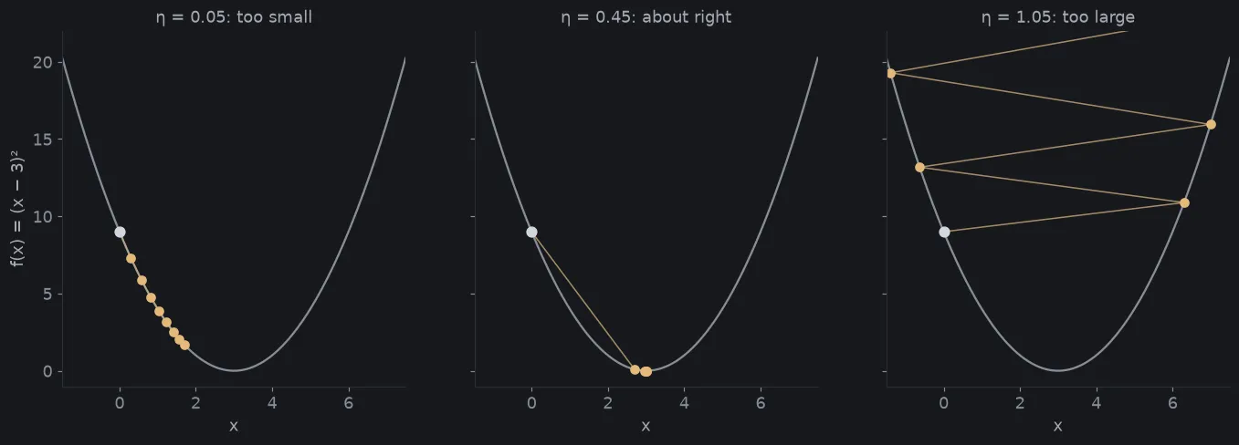
With a learning rate that is too small, the algorithm goes the right way but at a snail’s pace. Just right, it reaches the bottom in a few steps. Too large, each step overshoots the bottom onto the other slope, higher than before, and it flies further away with every step.
Choosing the learning rate is one of the most annoying parts of training real models, because we don’t know the shape of the mountain in advance.
Example: guessing how a taxi fare is computed
Now a problem with two parameters and more “real” data. Suppose you recorded the distance and fare of 30 taxi rides. You guess the company charges:
where is the flag-fall charge and is the price per km. But you don’t know and . The data is also noisy: traffic jams, rounding, surcharges. (Fares are in thousands of Vietnamese dong.)
The loss function is the mean squared error: for each pair , compute the predicted fare for every ride, take the difference from the real fare, square it and average. Gradient descent finds the that makes this number smallest on its own. The code below creates simulated data with a “true” fare of 12 thousand flag fall plus 15 thousand per km, then lets the algorithm guess:
import random
# Simulated data: 30 taxi rides. True fare = 12k flag fall + 15k per km, plus noise (traffic, rounding...)rng = random.Random(7)km = [round(rng.uniform(1, 20), 1) for _ in range(30)]fare = [12 + 15 * x + rng.gauss(0, 6) for x in km]n = len(km)
def loss(b, w):  # mean squared error    return sum((b + w * x - y) ** 2 for x, y in zip(km, fare)) / n
b, w, lr = 0.0, 0.0, 0.005          # start at 0; lr is the learning ratefor step in range(1, 5001):    err = [b + w * x - y for x, y in zip(km, fare)]    grad_b = 2 * sum(err) / n                               # derivative of the loss with respect to b    grad_w = 2 * sum(e * x for e, x in zip(err, km)) / n    # derivative of the loss with respect to w    b, w = b - lr * grad_b, w - lr * grad_w                 # step downhill    if step in (1, 10, 100, 1000, 5000):        print(f"step {step:>6}: flag fall {b:6.2f}k, rate {w:5.2f}k/km, loss {loss(b, w):8.2f}")
# Compare with the exact formula for linear regression (least squares)mx, my = sum(km) / n, sum(fare) / nw_ols = sum((x - mx) * (y - my) for x, y in zip(km, fare)) / sum((x - mx) ** 2 for x in km)print(f"exact formula: flag fall {my - w_ols * mx:6.2f}k, rate {w_ols:5.2f}k/km")
step 1: flag fall 1.38k, rate 16.07k/km, loss 77.28step 10: flag fall 1.67k, rate 15.74k/km, loss 65.76step 100: flag fall 4.41k, rate 15.51k/km, loss 48.88step 1000: flag fall 12.83k, rate 14.80k/km, loss 24.75step 5000: flag fall 13.48k, rate 14.75k/km, loss 24.63exact formula: flag fall 13.48k, rate 14.75k/kmAfter 5,000 steps, gradient descent finds a flag fall of 13.48 thousand and a rate of 14.75 thousand per km, matching exactly the answer from the linear regression formula. The numbers are not exactly 12 and 15 because the data is noisy: this is the best possible explanation of the data, not the “truth” behind it.
For a straight-line problem we have a direct formula, so gradient descent isn’t really needed. But for a neural network with billions of parameters and countless nonlinear layers stacked on top of each other, no such formula exists. Walking down the mountain is the only way.
A long, narrow valley
Look closely at the output and something is odd. The rate is nearly right after one step, while the flag fall takes about a thousand steps. Why do the two parameters learn at such different speeds?
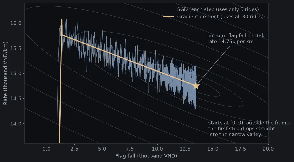
Figure 2 answers that question. It is a height map of the loss over the two parameters, drawn with contour lines like a topographic map. Its shape is not a round bowl but a long, narrow valley.
The reason lies in the data. Distances range from 1 to 20 km, so changing the rate a little changes the fare a lot: in the rate direction, the slope is very steep. The flag fall only adds a fixed amount: in that direction, the slope is very gentle. Gradient descent steps straight down the steep direction, lands right on the valley floor, then has to shuffle in tiny steps along a nearly flat floor to reach the bottom.
We can’t just raise the learning rate to go faster, because in the steep direction a large step would throw the algorithm off, like the case above. This problem is very common in practice, and there are two usual remedies: normalizing the data so every direction has a similar slope, and smarter variants of gradient descent that we will meet later.
Billions of dimensions: backpropagation
With two parameters, derivatives are easy to compute by hand. With a neural network of dozens of layers and billions of parameters, computing the derivative of the loss with respect to every parameter sounds like an enormous amount of work.
The solution comes from the chain rule of calculus. A neural network is a chain of transformations: the output of one layer is the input of the next. The effect of a parameter in the first layer on the final result is the product of small effects through each layer. Computing backwards from the end to the start, we can reuse the results for later layers to compute those for earlier layers, instead of starting over for every parameter.
This technique is called backpropagation. The idea of computing derivatives in reverse had appeared before, but the 1986 paper by Rumelhart, Hinton and Williams in Nature showed that it lets multi-layer neural networks learn useful representations, and made it popular[3]. Thanks to backpropagation, computing the gradient for all parameters costs only a few times as much as an ordinary prediction.
Gradient descent says which way to go. Backpropagation says where that way is, at an acceptable cost. The two ideas almost always go together.
No need to look at all the data: SGD
There is one more obstacle. The loss function is the average error over all the training data. For a language model, that data can be trillions of words. Computing the exact gradient over all of it just to take one step is far too expensive.
The solution: at each step, take only a small random group of data (a mini-batch), compute the gradient on that group, and step along it. The gradient from a small group is not exact, but on average it points the right way. This is stochastic gradient descent (SGD). Its mathematical foundations trace back to Robbins and Monro’s 1951 work on stochastic approximation[4].
In Figure 2, the blue line is SGD for the taxi problem, each step using only 5 of the 30 rides. It wobbles and jerks back and forth, but still makes its way close to the bottom. And each of its steps is many times cheaper than a step using all the data.
Interestingly, this “wobbling” is not purely a weakness. On the rugged mountains of neural networks, a little random noise can help the algorithm escape small dips or flat regions where exact gradient descent easily gets stuck.
The terrain of neural networks
The loss of the taxi problem is a simple valley: it has a single bottom. The loss of a neural network is different: it lives in a space of billions of dimensions, with countless hills, pits and passes.
The natural worry is that the algorithm gets stuck in a local minimum, a small pit on the mountainside that looks like the bottom but isn’t. A 2014 study by Dauphin and colleagues suggests a different picture: in high-dimensional spaces, “flat” points with high error are usually not pits but saddle points: curving down in some directions and up in others, like a saddle or a pass between two peaks[5]. There, the gradient is close to zero, and the algorithm can slow down for a long time even though a way down still exists.
Two improvements help gradient descent cross terrain like that:
- Momentum: instead of looking only at the local slope, the algorithm remembers the direction of previous steps, like a ball rolling downhill and picking up speed. The ball rolls across flat regions, and in a narrow valley like the taxi problem, the back-and-forth oscillations across the slopes cancel out while the movement along the valley floor adds up.
- Adam, proposed by Kingma and Ba in 2014, combines momentum with automatically adapting the learning rate for each parameter, based on the size of its recent gradients[6]. Parameters with large, erratic gradients take shorter steps; parameters with small gradients take longer ones. That is exactly the cure for the “long, narrow valley” problem. Adam and its variants are now the default choice for training a great many deep learning models.
Whatever the improvements, the core is still Cauchy’s line: compute the slope, step the other way.
Optimizing too well is also a trap
Gradient descent is very good at doing exactly what it is told: finding the parameters that minimize the loss on the training data. But that is not what we really want. We want the model to work well on data it has never seen.
The two goals can come apart. A big enough model can memorize even the random details of its training data, such as ride number 17 happening to hit a traffic jam. This is called overfitting: the loss on training data is very low, but the model predicts poorly on new data.
That is why in practice a part of the data is always held out for validation and never used for training. When the validation error starts rising while the training error keeps falling, it is a sign to stop. The mountain gradient descent walks down is only an approximate map of the real world, and going too deep on that map can take you away from reality.
Every step down the mountain costs electricity
On paper, gradient descent is one line of math. In practice, with a large model, each step is a round of computation on thousands of GPUs, and training can take hundreds of thousands of steps over many weeks. According to its authors, training GPT-3 took about floating-point operations[2], and the models that came after are much larger.
That is why AI training is tied to the story of electricity, cooling and power grids in the article AI needs more than chips (in Vietnamese). At this scale, every improvement that gets gradient descent to the bottom a few percent faster saves thousands of GPU hours.
An algorithm from 1847
Back to the opening question: how do you choose 175 billion numbers?
The answer is not an algorithm so clever that it sees the solution. It is a very humble procedure: stand where you are, measure the slope, take a small step down, and repeat hundreds of thousands of times. Backpropagation measures the slope quickly. SGD makes each step cheap. Momentum and Adam get through difficult terrain. Validation data tells us when to stop.
Gradient descent does not stand alone. Model architecture, data and hardware matter just as much. But almost every modern AI model, from image recognition to large language models, is trained with gradient descent or one of its variants. Cauchy’s idea from nearly two centuries ago is still running, billions of times a second, in the world’s largest data centers.
Tài liệu tham khảo
- [1]Augustin-Louis Cauchy. Méthode générale pour la résolution des systèmes d'équations simultanées. Comptes Rendus de l'Académie des Sciences, 25, 536–538, 1847.
- [2]Tom B. Brown et al.. Language Models are Few-Shot Learners. arXiv:2005.14165, 2020.
- [3]David E. Rumelhart, Geoffrey E. Hinton and Ronald J. Williams. Learning representations by back-propagating errors. Nature, 323, 533–536, 1986.
- [4]Herbert Robbins and Sutton Monro. A Stochastic Approximation Method. The Annals of Mathematical Statistics, 22(3), 400–407, 1951.
- [5]Yann Dauphin et al.. Identifying and attacking the saddle point problem in high-dimensional non-convex optimization. arXiv:1406.2572, 2014.
- [6]Diederik P. Kingma and Jimmy Ba. Adam: A Method for Stochastic Optimization. arXiv:1412.6980, 2014.