Image search: snap a pair of shoes, find that exact model
How image search works: AI turns each picture into a list of numbers, then finds the "nearest" ones among billions without comparing them one by one.
Mục lục
You spot a nice pair of shoes in the street, take a photo, and a few seconds later a shopping app shows that exact model, along with similar ones. Nobody typed “white high-sole trainers with blue trim”. Image search works in two steps: an AI model turns every picture into a list of numbers, so that similar pictures get similar numbers; then the system finds the lists closest to your photo, among millions or billions of pictures, without comparing it with each one.
This article covers those two steps: why a picture can become a point in space, why finding the “nearest neighbours” among billions of points is hard, and the tricks that make it run in a few milliseconds. The same technique is also behind AI chatbots that answer from your own documents.
A picture becomes a list of numbers
A computer does not “see” a pair of shoes. It sees millions of pixels, each of them three numbers for red, green and blue. Comparing two pictures pixel by pixel is useless: the same pair of shoes photographed from another angle, in other light, gives completely different numbers.
The modern approach is to use a neural network trained on a huge number of pictures to turn each picture into a list of a few hundred numbers, called an embedding. The network is trained so that pictures of the same thing produce nearby lists and different pictures produce distant ones. Each picture thus becomes a point in a space with a few hundred dimensions: white trainers cluster in one place, leather handbags in another, and two photos of the same pair of shoes sit side by side whatever the angle.
The big step forward in 2021 was OpenAI’s CLIP model, which learned from about 400 million image–caption pairs collected from the internet. CLIP puts images and text in the same space: a photo of a dog and the words “a dog” sit close together[1]. That is why you can type “a cat sitting on a suitcase” to search your photo library without anyone labelling each picture.
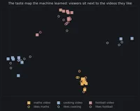
The idea of “every item is a point, similar items sit close together” is the same taste map from the article on how YouTube and TikTok recommend videos, except that the points here are pictures instead of viewers.
Nearest neighbour search: easy to say, hard to do
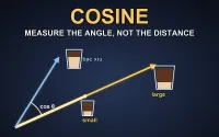
Once every picture is a point, the question “which picture is most like this one?” becomes: which point is closest to this point? This is the nearest neighbour search problem. Closeness is usually measured by the angle between the two lists of numbers, a measure called cosine similarity.
The honest way is to measure the distance from your picture to every picture in the store, then pick the ten closest. With a thousand pictures it is instant. With a billion pictures of a few hundred numbers each, every search takes hundreds of billions of multiplications, and the system has to answer thousands of people every second.
In the article on binary search and database indexes, an index makes lookups fast because data can be sorted along one axis. But points in a space with hundreds of dimensions cannot be put in a single line: two pictures that are close along one dimension can be far apart along another. Different ideas are needed.
Three tricks for searching billions of pictures
All three tricks accept one thing: approximately right is good enough. If the true best match is the first pair of shoes and the system returns a second pair that looks almost identical, the user cannot tell the difference. Trading a little accuracy for hundreds of times the speed is called approximate nearest neighbour search.
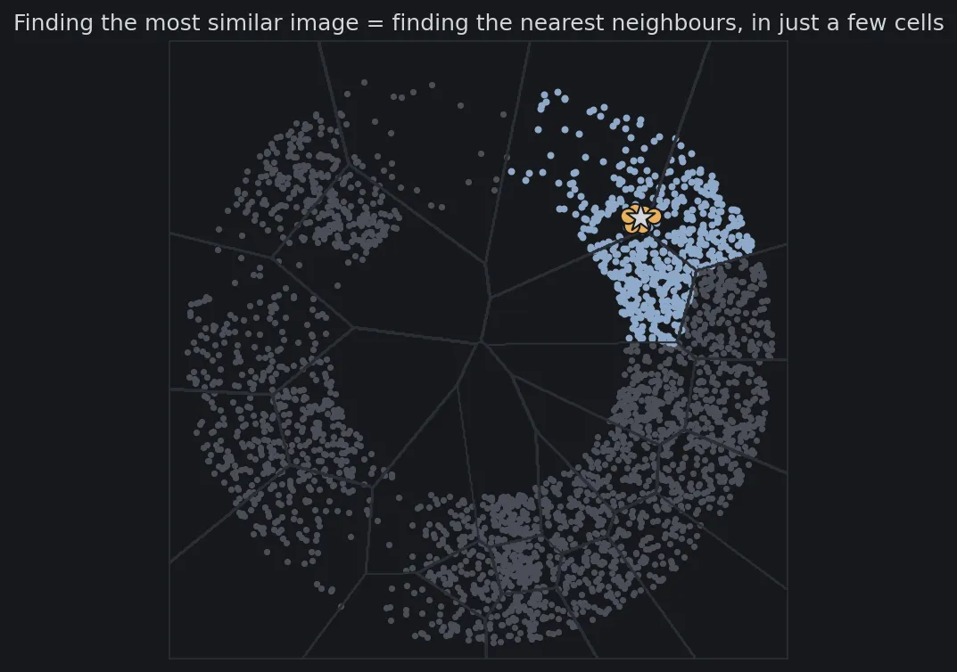
Split into cells. First, group the pictures into a few thousand clusters, each with a representative point. When searching, compare your picture only with the representatives, pick the few closest clusters, and only then compare carefully with the pictures inside those clusters. The image at the top of this article shows the idea on a plane: the star is the picture being searched for, only three cells near it are opened, and the rest are skipped. At the end of the article, a simulation with 50,000 simulated pictures shows that scanning only 8% of the data already finds 91% of the ten most similar pictures.
Compress each picture. A list of a few hundred real numbers takes thousands of bytes. Product quantization cuts the list into many short pieces, then replaces each piece with the code of the nearest pattern in a small table of patterns. Each picture shrinks to a few dozen bytes, so a billion pictures fit in memory, and distances are computed approximately by table lookups[5].
Follow a graph. Connect each picture to the few pictures nearest to it, forming a network. To search, start from any picture and jump to whichever neighbour is closer to the target, until you cannot get any closer. The HNSW method also arranges the network in layers: sparse upper layers for long jumps, dense lower layers for a careful search, like taking the motorway first and then the side streets[4].
Meta’s FAISS library combines these techniques and runs them on GPUs. The title of the paper introducing it says everything about the scale: similarity search at the billion scale[3].
In the real world: from Pinterest to AI chatbots
In 2015 Pinterest described its visual search system: a user selects part of a picture, such as a lamp in a photo of a living room, and the system finds pictures with similar objects. The features of each picture are extracted with a neural network, then the closest pictures are found in its huge image store[2].
The biggest application today may not involve pictures at all. When an AI chatbot answers from a company’s documents, it often works like this: cut the documents into passages, turn each passage into an embedding, and store them in a vector database. When you ask a question, the question is turned into an embedding too, the system finds the closest passages, and hands them to the language model to read before it answers. This is called retrieval-augmented generation (RAG)[6]. Here, “find the nearest neighbours” decides whether the chatbot reads the right documents.
Running it for millions of users
Turning the idea into a real system raises a few design questions.
- How accurate to be. Opening more cells is more accurate but slower (Figure 1). Each system picks its own balance: when shopping, being slightly off is fine; when searching for duplicate pictures to block prohibited content, more accuracy is needed.
- Filtering by conditions. Users want “shoes like these, under 40 dollars, in size 40”. Combining distance search with filters on price, size and stock is one of the hardest parts of a vector database.
- Updates. Millions of new pictures arrive every day. Some indexes, like cells, have to be rebuilt periodically when the data changes a lot; graphs make it easier to add new points but use more memory.
- Splitting up. A billion vectors do not fit on one machine. The data is spread over many machines, each searches its own part, and the results are merged. How to add or remove machines without moving all the data again is a problem of its own, familiar in every distributed system.
- Embeddings and index go together. Switching to a newer, better AI model means every picture’s embedding must be recomputed and the index rebuilt from scratch, because the numbers from the old and new models cannot be compared.
Run it yourself: how much do you need to scan?
The Python below simulates 50,000 “pictures” from 300 groups of objects, each picture a 64-dimensional vector, plus 200 query pictures. It finds the ten most similar pictures by scanning everything (the exact answer), then with a cell index (splitting the data into 100 cells with the k-means algorithm), opening more and more cells. Each time it measures the share of data scanned and the share of correct results found. This is simulated data to show the shape of the trade-off; the exact numbers on real pictures will differ. You need numpy and matplotlib.
import numpy as npimport matplotlib.pyplot as plt
plt.rcParams.update({"figure.facecolor": "#16181c", "axes.facecolor": "#16181c", "text.color": "#d4d7dc",                     "axes.edgecolor": "#2a2e35", "xtick.color": "#878d97", "ytick.color": "#878d97", "font.size": 12})rng = np.random.default_rng(2026)

def make_data(n, centers, noise):    """n simulated "image" vectors: each image belongs to a group (shoes, bags, shirts...) and sits around its centre."""    labels = rng.integers(0, len(centers), n)    x = centers[labels] + rng.normal(0, noise, (n, centers.shape[1]))    return x / np.linalg.norm(x, axis=1, keepdims=True)    # normalise: compare by angle (cosine)

def kmeans(x, k, steps=20):    c = x[rng.choice(len(x), k, replace=False)]    for _ in range(steps):        assign = np.argmax(x @ c.T, axis=1)                # assign each vector to its nearest centre        for j in range(k):            if np.any(assign == j):                c[j] = x[assign == j].mean(0)        c /= np.linalg.norm(c, axis=1, keepdims=True)    return c, np.argmax(x @ c.T, axis=1)

# ── Experiment: 50,000 "images", each a 64-dimensional vector; 200 queries; find the 10 most similar images.N, DIM, TOPK, NLIST = 50_000, 64, 10, 100groups = rng.normal(0, 1, (300, DIM))                       # 300 groups of objectsdata = make_data(N, groups, 1.2)queries = make_data(200, groups, 1.2)                       # the photo you take also belongs to a group already in the storeexact = np.argsort(-(queries @ data.T), axis=1)[:, :TOPK]  # scan everything: exact but expensive
centroids, cell = kmeans(data, NLIST)                       # IVF index: split the data into 100 cellsmembers = [np.nonzero(cell == j)[0] for j in range(NLIST)]results = []for nprobe in [1, 2, 4, 8, 16, 32, 100]:    recall, scanned = 0, 0    for q, truth in zip(queries, exact):        cells = np.argsort(-(centroids @ q))[:nprobe]       # open only the nprobe cells nearest the query        cand = np.concatenate([members[j] for j in cells])        top = cand[np.argsort(-(data[cand] @ q))[:TOPK]]        recall += len(set(top) & set(truth)) / TOPK        scanned += len(cand)    results.append((nprobe, scanned / len(queries) / N, recall / len(queries)))    print(f"open {nprobe:>3} cell(s): scan {scanned / len(queries) / N:6.1%} of the data, find {recall / len(queries):6.1%} of the 10 most similar images")
# Figure 1: how little data can we scan and still find the right images.fig, ax = plt.subplots(figsize=(9, 5))xs = [100 * s for _, s, _ in results]ys = [100 * r for _, _, r in results]ax.plot(xs, ys, "o-", color="#e8b05a", lw=2.5, ms=8)for (p, s, r), x, y in zip(results, xs, ys):    ax.annotate(f"open {p} cell" + ("s" if p > 1 else ""), (x, y), xytext=(8, -16), textcoords="offset points", color="#a4a9b2", fontsize=10)ax.set_xscale("log")ax.set_xticks([1, 2, 4, 8, 16, 32, 100], ["1%", "2%", "4%", "8%", "16%", "32%", "100%"])ax.minorticks_off()ax.set_xlabel("share of the data scanned (log scale)", color="#a4a9b2")ax.set_ylabel("found among the 10 most similar images (%)", color="#a4a9b2")ax.set_title("Cell index: scan a small part, still find nearly the right answer", color="#d4d7dc", fontsize=12)ax.grid(color="#22262c")fig.savefig("quet-it-van-tim-dung-en.png", dpi=150, bbox_inches="tight")
# Cover image: the same idea on a plane — data split into cells, a query opens only the few nearest cells.pts = make_data(3000, rng.normal(0, 1, (12, 2)), 0.25) * rng.uniform(0.5, 1.0, (3000, 1))c2 = pts[rng.choice(len(pts), 24, replace=False)]for _ in range(15):    a2 = np.argmin(((pts[:, None] - c2[None]) ** 2).sum(-1), axis=1)    c2 = np.array([pts[a2 == j].mean(0) if np.any(a2 == j) else c2[j] for j in range(len(c2))])q2 = np.array([0.55, 0.45])open_cells = np.argsort(((c2 - q2) ** 2).sum(-1))[:3]gx, gy = np.meshgrid(np.linspace(-1.05, 1.05, 500), np.linspace(-1.05, 1.05, 500))grid_cell = np.argmin(((np.stack([gx, gy], -1)[..., None, :] - c2) ** 2).sum(-1), axis=-1)fig, ax = plt.subplots(figsize=(9, 6))ax.contour(gx, gy, grid_cell, levels=np.arange(len(c2)) + 0.5, colors="#2a2e35", linewidths=1)inside = np.isin(a2, open_cells)ax.scatter(*pts[~inside].T, s=6, color="#4a4e57")ax.scatter(*pts[inside].T, s=8, color="#8fa9c9")near = np.argsort(((pts - q2) ** 2).sum(-1))[:10]ax.scatter(*pts[near].T, s=70, color="#e8b05a", edgecolors="#16181c", zorder=3)ax.scatter(*q2, marker="*", s=260, color="#d4d7dc", edgecolors="#16181c", zorder=4)ax.set_xticks([]); ax.set_yticks([]); ax.set_aspect("equal")ax.set_xlim(-1.05, 1.05); ax.set_ylim(-1.05, 1.05)ax.set_title("Finding the most similar image = finding the nearest neighbours, in just a few cells", color="#d4d7dc", fontsize=12)fig.savefig("hang-xom-gan-nhat-en.png", dpi=150, bbox_inches="tight")
open 1 cell(s): scan 1.0% of the data, find 76.2% of the 10 most similar imagesopen 2 cell(s): scan 2.1% of the data, find 81.9% of the 10 most similar imagesopen 4 cell(s): scan 4.1% of the data, find 86.0% of the 10 most similar imagesopen 8 cell(s): scan 8.0% of the data, find 91.2% of the 10 most similar imagesopen 16 cell(s): scan 16.0% of the data, find 94.9% of the 10 most similar imagesopen 32 cell(s): scan 32.2% of the data, find 97.9% of the 10 most similar imagesopen 100 cell(s): scan 100.0% of the data, find 100.0% of the 10 most similar images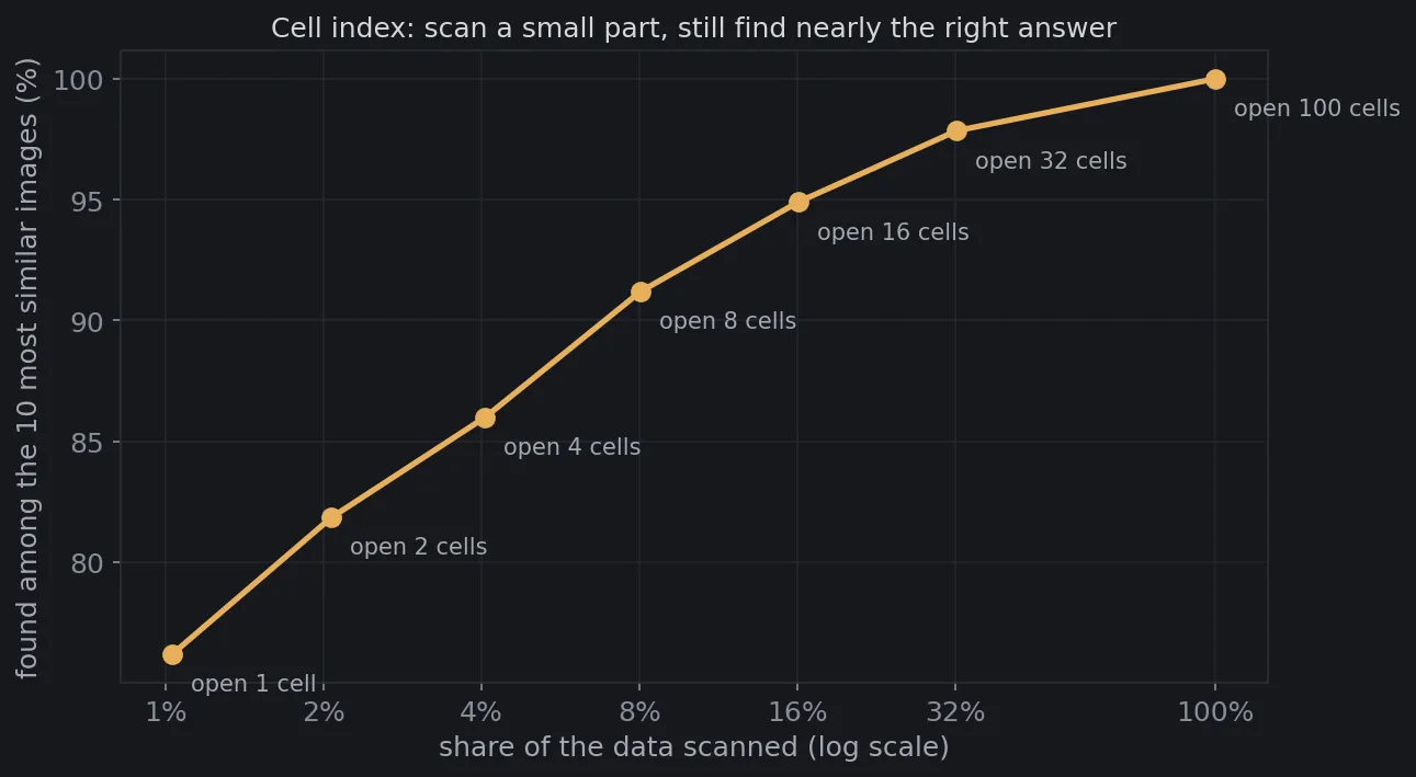
Opening just one cell, that is scanning 1% of the data, the system already finds about three quarters of the ten most similar pictures. Opening 8 cells (scanning 8%) finds 91%, about twelve times faster than scanning everything. The pictures it misses usually sit at the edge of a neighbouring cell, exactly where a cell boundary cuts through a group of similar pictures, as you can see in the image at the top of the article.
You can change NLIST (the number of cells) or the noise 1.2 to see the curve shift: the more clearly the data forms groups, the more effective a cell index becomes.
Similarity is a distance
Image search, video recommendations, chatbots that read documents: three things that sound very different all rest on the same idea. Turn everything into points in a space so that “similar” means “close”, then find the neighbours very fast, accepting almost exactly right instead of exactly right. Next time an app finds the exact pair of shoes you just photographed, behind it is a small star among billions of points, with a few cells opened around it.
Free geometry illustrations for students and teachers: EyeViz.
Tài liệu tham khảo
- [1]Alec Radford et al.. Learning Transferable Visual Models From Natural Language Supervision (CLIP). ICML 2021, 2021.
- [2]Yushi Jing et al.. Visual Search at Pinterest. KDD ’15, 2015.
- [3]Jeff Johnson, Matthijs Douze and Hervé Jégou. Billion-scale similarity search with GPUs. IEEE Transactions on Big Data, 2019.
- [4]Yu. A. Malkov and D. A. Yashunin. Efficient and robust approximate nearest neighbor search using Hierarchical Navigable Small World graphs. IEEE Transactions on Pattern Analysis and Machine Intelligence, 42(4), 2020.
- [5]Hervé Jégou, Matthijs Douze and Cordelia Schmid. Product Quantization for Nearest Neighbor Search. IEEE Transactions on Pattern Analysis and Machine Intelligence, 33(1), 2011.
- [6]Patrick Lewis et al.. Retrieval-Augmented Generation for Knowledge-Intensive NLP Tasks. NeurIPS 2020, 2020.