Binary search: from a guessing game to database indexes
Thirty comparisons find one row among a billion. But databases skip textbook binary search: they use B-trees, where each step is a disk read.
Mục lục
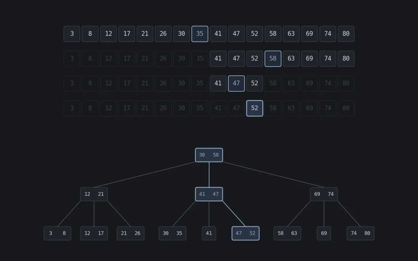
I think of a number from 1 to 100; you guess, and I only answer “higher” or “lower”. First-time players guess at random: 37, then 80, then 52. Experienced players always start with 50, then 25 or 75, each time ruling out half of what remains. They never need more than 7 guesses.
That strategy is called binary search. It is probably the first algorithm computer science students learn, and it is also the algorithm running quietly behind every SELECT ... WHERE id = 42 you send to a database. But databases do not use it the way the textbook teaches. This article goes from the guessing game to that point, and explains why.
Halve, then halve again
Binary search needs only one condition: the data must already be sorted. To find key in an array of elements:
- Look at the element in the middle of the current range.
- If it is smaller than , then (if present) can only be in the right half. Drop the left half.
- Otherwise, drop the right half.
- Repeat until the range is empty.
Each step removes half, so after steps only elements remain. The range shrinks to a single element once , that is, after about
steps. That number grows unbelievably slowly:
| Elements | Linear scan (average) | Binary search (maximum) |
|---|---|---|
| 100 | 50 | 7 |
| 1,000,000 | 500,000 | 20 |
| 1,000,000,000 | 500,000,000 | 30 |
| 8 billion (world population) | 4 billion | 33 |
Making the data a thousand times bigger costs only about 10 more steps, because . This is why every storage system tries to keep data ordered in one way or another: order turns a linear problem into a logarithmic one.
The simplest algorithm everyone gets wrong
As simple as it sounds, binary search is notoriously hard to get right. In Programming Pearls, Jon Bentley recounts giving this task to professional programmers in his courses, with plenty of time, and only about one in ten handed in a correct program[1].
The usual bugs sit at the boundaries: the loop runs one time too many or too few, updating hi = mid instead of hi = mid - 1 makes the loop never terminate, or the wrong position is returned when the key appears several times.
The most famous bug is subtler. In 2006, Joshua Bloch, who wrote the binary search in Java’s standard library, announced that it had been broken for nine years[2]. The culprit was the line computing the midpoint, mid = (lo + hi) / 2. With an array of more than about a billion elements, the sum lo + hi exceeds the limit of a 32-bit integer () and overflows into a negative number. The fix is mid = lo + (hi - lo) / 2. Bloch pointed out that the very version Bentley proved correct in Programming Pearls had the same bug: the proof was right for mathematical integers, but computers do not use mathematical integers.
The lower_bound version matters more than the “find the exact value” version, because it also answers “if is not there, where would it be?”. Databases need exactly that question for range queries, as we will see below.
Why don’t databases just use a sorted array?
If binary search is that good, why doesn’t a database store a table as one big file sorted by key and search that? Two reasons.
First: adding data is very expensive. Inserting a row in the middle of a sorted array means shifting every row after it. With a billion rows, each INSERT could rewrite hundreds of megabytes.
Second, and more important: disks do not read one row at a time. Databases read and write in units of pages, fixed-size blocks: 8 KB in PostgreSQL[5], 16 KB by default in MySQL’s InnoDB[7]. To compare with row mid, the database must read the whole page containing that row. And each binary search step jumps far from the previous position, so almost every step lands on a different page, which is a random read from disk.
A comparison in RAM takes a few nanoseconds. A random read from an SSD takes on the order of a hundred microseconds, and from a spinning hard disk on the order of ten milliseconds (these are orders of magnitude for illustration; a specific machine will differ). In other words, reading from disk is tens of thousands to millions of times slower than comparing. For a database, the thing to count is not comparisons, but pages read.
Figure 1 counts exactly that for three ways of finding a row, assuming 100 rows per page:
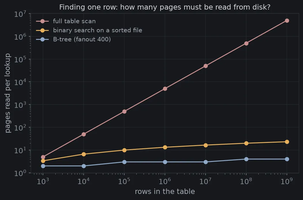
With a billion rows, binary search on a sorted file reads about 23 pages. Only the last few steps, once the range fits inside a single page, cost no extra reads. The B-tree needs just 4 pages.
B-trees: divide by a hundred instead of by two
B-trees were published by Rudolf Bayer and Edward McCreight in the early 1970s[3]. By the end of that decade a survey already called them “ubiquitous”[4], and today they are still the default index in PostgreSQL, MySQL, SQLite, Oracle and SQL Server.
The core idea is very close to binary search. Binary search divides the range in two at each step, and each step costs one disk read. So if each disk read brings back a whole 8 KB page anyway, why not use all of that page to divide the range into several hundred parts?
Each B-tree node is a page. An inner node holds a few hundred sorted keys, interleaved with pointers to child nodes: every key smaller than the first key is in the first branch, every key between the first and second keys is in the second branch, and so on. The bottom level holds the leaves, which contain the actual data (or pointers to the rows).
The number of branches per node is called the fanout, written . A tree levels tall holds about keys, so holding keys takes only
levels. With , , so the height is nearly nine times smaller than a binary tree’s. A billion rows need just four levels.
One more detail makes the real number even smaller. Those four levels are not equal: the root level is one page, the second a few dozen pages, the third a few tens of thousands of pages. The top three levels together are only about 200 MB with 8 KB pages, small enough to sit entirely in the database’s buffer cache. In practice, finding one row among a billion usually costs one or two actual disk reads.
Binary search is still there, inside every page
B-trees do not replace binary search. They move it to the cheapest possible place: inside a page that is already in RAM. On reaching a node, the database needs to find which of the few hundred branches the key falls into, and it does so with binary search over the node’s keys.
- PostgreSQL does this in the function
_bt_binsrch. It returns the first position with a key the search key, which is exactlylower_bound, with the invariant written right in the comment[6]. - InnoDB uses a variant. The rows in a page are linked into a list in key order, and at the end of the page there is a “page directory” of slots, each covering about 4 to 8 rows. InnoDB binary searches the directory to find the right group, then walks a few rows sequentially within it[8]. This makes inserts cheaper: most inserts do not need to shift anything in the directory.
Interestingly, the total number of comparisons barely changes. Binary search over a billion rows needs about 30 comparisons. A four-level B-tree, binary searching a few hundred keys at each level, also costs about 30 comparisons. A B-tree does not reduce comparisons, it reduces disk reads. In a world where one disk read costs as much as thousands of comparisons, that is the only thing worth optimizing.
Adding data without shifting the whole table
B-trees also solve the first problem. Each leaf page is left partly empty. Inserting a new row only rearranges one page. When a page is full, it splits into two half-full pages, and the parent node gains one key. If the parent is full too, the split continues upward. The tree always stays balanced (every leaf at the same depth), yet each insert touches only a few pages.
Range queries, and what indexes cannot do
Thinking of an index as “binary search over ordered data” answers many practical questions about SQL performance.
Range queries. For WHERE created_at BETWEEN '2026-09-01' AND '2026-09-30', the database uses lower_bound to descend to the leaf holding the first row 2026-09-01, then walks sideways along the leaves (B-tree leaves are linked in order) until it meets a value past 2026-09-30. The cost is a few pages to locate the start plus the pages holding the results. ORDER BY created_at LIMIT 20 is cheap for the same reason: the data is already sorted in the index.
Composite indexes and the “leftmost prefix” rule. An index on (last_name, first_name) is sorted like a phone book: by last name first, then by first name within the same last name. Finding “Smith, John” or everyone named “Smith” is a binary search over a contiguous range. But finding everyone whose first name is “John” is not: people named John are scattered all over the phone book, with no contiguous range to halve. So column order in a composite index matters: columns usually filtered with = should come first.
LIKE and functions on columns. WHERE email LIKE 'an%' can use the index, because every email starting with an sits together in the order. WHERE email LIKE '%@gmail.com' cannot, because the ending does not determine the order. Likewise, WHERE lower(email) = '...' cannot use an index on email: the index is sorted by email, not by lower(email). For that you need an index on the expression itself.
LSM-trees: binary search over files that are never modified
B-trees modify pages in place, which is costly when a system writes a lot. Write-optimized databases such as RocksDB, Cassandra and ScyllaDB use a different idea: the LSM-tree (log-structured merge-tree)[9].
New data is written to a table in RAM. When the table fills up, it is flushed to disk as a file that is sorted and never modified again (usually called an SSTable). Over time, small files are merged (compaction) into larger ones, also sorted. Each file has a sparse index at the end, storing the first key of each data block.
Finding a key in an SSTable is binary search again: search the sparse index to find which block the key is in, then read just that block. Since there are many files, a lookup may have to check several. To avoid that, each file usually comes with a Bloom filter, a probabilistic structure that can answer “this key is definitely not in the file” without reading the file. The article Bloom filter: how sites instantly know a username is taken explains how it works.
Count the pages yourself
The Python below produces Figure 1. It simulates a table of rows, row with key , 100 rows per page. For binary search, it runs 1,000 lookups of random keys and counts the distinct pages each one touches. For the B-tree, it builds the tree bottom-up and counts the levels. All you need is matplotlib.
The parameters (100 rows per page, 400 branches per node) are reasonable estimates for 8 KB pages, not measurements of a specific database. You can change ROWS_PER_PAGE or FANOUT to see how the B-tree line moves.
import random
import matplotlib.pyplot as plt
plt.rcParams.update({"figure.facecolor": "#16181c", "axes.facecolor": "#16181c", "text.color": "#d4d7dc",                     "axes.edgecolor": "#2a2e35", "xtick.color": "#878d97", "ytick.color": "#878d97", "font.size": 12})random.seed(2026)  # Fixed seed: every run gives the same result.
ROWS_PER_PAGE = 100   # rows that fit in an 8 KB page (estimate, rows of about 80 bytes)FANOUT = 400          # children per B-tree node (key + pointer of about 20 bytes)

def binary_search_pages(n, key):    """Binary search over a sorted file. Row i has key 2i.    Returns (comparisons, distinct pages read from disk)."""    lo, hi = 0, n    compares, pages = 0, set()    while lo < hi:        mid = lo + (hi - lo) // 2          # not (lo + hi) // 2: avoids overflow in other languages        pages.add(mid // ROWS_PER_PAGE)    # the page that row mid lives on        compares += 1        if 2 * mid < key:            lo = mid + 1        else:            hi = mid    return compares, len(pages)

def btree_height(n):    """Build a B-tree bottom-up: leaves hold rows, each level above groups FANOUT nodes below.    A lookup reads exactly one page per level, so pages = levels."""    nodes, height = -(-n // ROWS_PER_PAGE), 1    while nodes > 1:        nodes, height = -(-nodes // FANOUT), height + 1    return height

sizes = [10**k for k in range(3, 10)]scan, bsearch, btree = [], [], []print(f"{'rows':>14} {'scan':>12} {'compares':>8} {'binary search':>14} {'B-tree':>7}")for n in sizes:    trials = [binary_search_pages(n, 2 * random.randrange(n)) for _ in range(1000)]    cmp_avg = sum(c for c, _ in trials) / len(trials)    pages_avg = sum(p for _, p in trials) / len(trials)    scan.append(n / ROWS_PER_PAGE / 2)     # on average a scan reads half the table before finding the row    bsearch.append(pages_avg)    btree.append(btree_height(n))    print(f"{n:>14,} {scan[-1]:>12,.0f} {cmp_avg:>8.1f} {pages_avg:>14.1f} {btree[-1]:>7}")
# Plot: pages read vs number of rows, both axes on a log scale.fig, ax = plt.subplots(figsize=(8, 4.8))ax.plot(sizes, scan, "o-", color="#c98f8f", ms=6, label="full table scan")ax.plot(sizes, bsearch, "o-", color="#e8b05a", ms=6, label="binary search on a sorted file")ax.plot(sizes, btree, "o-", color="#8fa9c9", ms=6, label=f"B-tree (fanout {FANOUT})")ax.set_xscale("log")ax.set_yscale("log")ax.set_xlabel("rows in the table", color="#a4a9b2")ax.set_ylabel("pages read per lookup", color="#a4a9b2")ax.grid(color="#22262c")ax.legend(frameon=False, labelcolor="#a4a9b2", fontsize=10, loc="upper left")ax.set_title("Finding one row: how many pages must be read from disk?", color="#d4d7dc", fontsize=12)fig.savefig("page-reads-en.png", dpi=150, bbox_inches="tight")
rows scan compares binary search B-tree 1,000 5 10.0 3.4 2 10,000 50 13.4 6.6 2 100,000 500 16.7 9.9 3 1,000,000 5,000 19.9 13.2 3 10,000,000 50,000 23.3 16.5 3 100,000,000 500,000 26.7 19.9 4 1,000,000,000 5,000,000 29.9 23.2 4The “compares” column matches : 10 comparisons for a thousand rows, 30 for a billion. The “binary search” column is always smaller by about , because the last few steps land in the same page. And the “B-tree” column barely moves: from a thousand to a billion rows, the page count only goes from 2 to 4.
One idea, many layers
Binary search teaches that order is precious: keep data ordered and searching becomes logarithmic. B-trees add a system design lesson: count the most expensive thing. Textbooks count comparisons, but databases count disk reads, and when you change what you count, the best algorithm changes too, from halving to dividing by a few hundred.
Next time a query is slow and EXPLAIN says Seq Scan, ask yourself: do the rows I need sit next to each other in some order? If they do, an index on exactly that order will turn millions of reads into a few. If they don’t, no index can save that query.
Tài liệu tham khảo
- [1]Jon Bentley. Programming Pearls (2nd edition), Column 4: Writing Correct Programs. Addison-Wesley, 2000.
- [2]Joshua Bloch. Extra, Extra - Read All About It: Nearly All Binary Searches and Mergesorts are Broken. Google Research Blog, 2006.
- [3]R. Bayer and E. McCreight. Organization and Maintenance of Large Ordered Indexes. Acta Informatica, 1(3), 173–189, 1972.
- [4]Douglas Comer. The Ubiquitous B-Tree. ACM Computing Surveys, 11(2), 121–137, 1979.
- [5]Database Page Layout. PostgreSQL Documentation.
- [6]nbtsearch.c — B-tree search in PostgreSQL (function _bt_binsrch). PostgreSQL Source Code.
- [7]InnoDB Startup Options and System Variables — innodb_page_size. MySQL 8.4 Reference Manual.
- [8]page0page.ic — the InnoDB page directory. MySQL Server Source Code Documentation.
- [9]P. O'Neil, E. Cheng, D. Gawlick and E. O'Neil. The Log-Structured Merge-Tree (LSM-Tree). Acta Informatica, 33(4), 351–385, 1996.