Bloom filter: how sites instantly know a username is taken
What a Bloom filter is: a few bits that answer "definitely not" or "maybe". How it works, how Akamai and Cassandra use it, sizing it, and when not to use one.
Mục lục
You type a new username, and almost instantly the site says: “This username is already taken”. Meanwhile the system may be holding hundreds of millions of accounts. One way to answer that fast, without digging through the whole database every time you type a letter, is a Bloom filter.
What is a Bloom filter? It is a tiny data structure, nothing more than a row of 0 and 1 bits, that answers the question “is this item already in the set?” with one of two replies: “definitely not” or “maybe”. It is never wrong about the first, and occasionally wrong about the second. In exchange for that occasional error, it costs only about 10 bits per item, no matter how long the item is: 100 million usernames fit in about 120 MB, small enough for the RAM of a phone.
The first half of this article needs no programming: it shows how a Bloom filter works, why a “maybe” answer is useful at all, and what companies like Akamai, Google and Cassandra use it for. The second half is for readers who want to go deeper: how to size one, the probability formula, how to answer a system design interview question with it, and a short program you can run to check the numbers yourself.
How does a Bloom filter work?
Picture a wall with 16 light switches, all off at the start. You also have a “name grinder”: feed it a name and it always points at exactly three switches, and the same name always gives the same three switches. In a computer, that grinder is called a hash function, a calculation that turns any string of characters into a number that looks random.
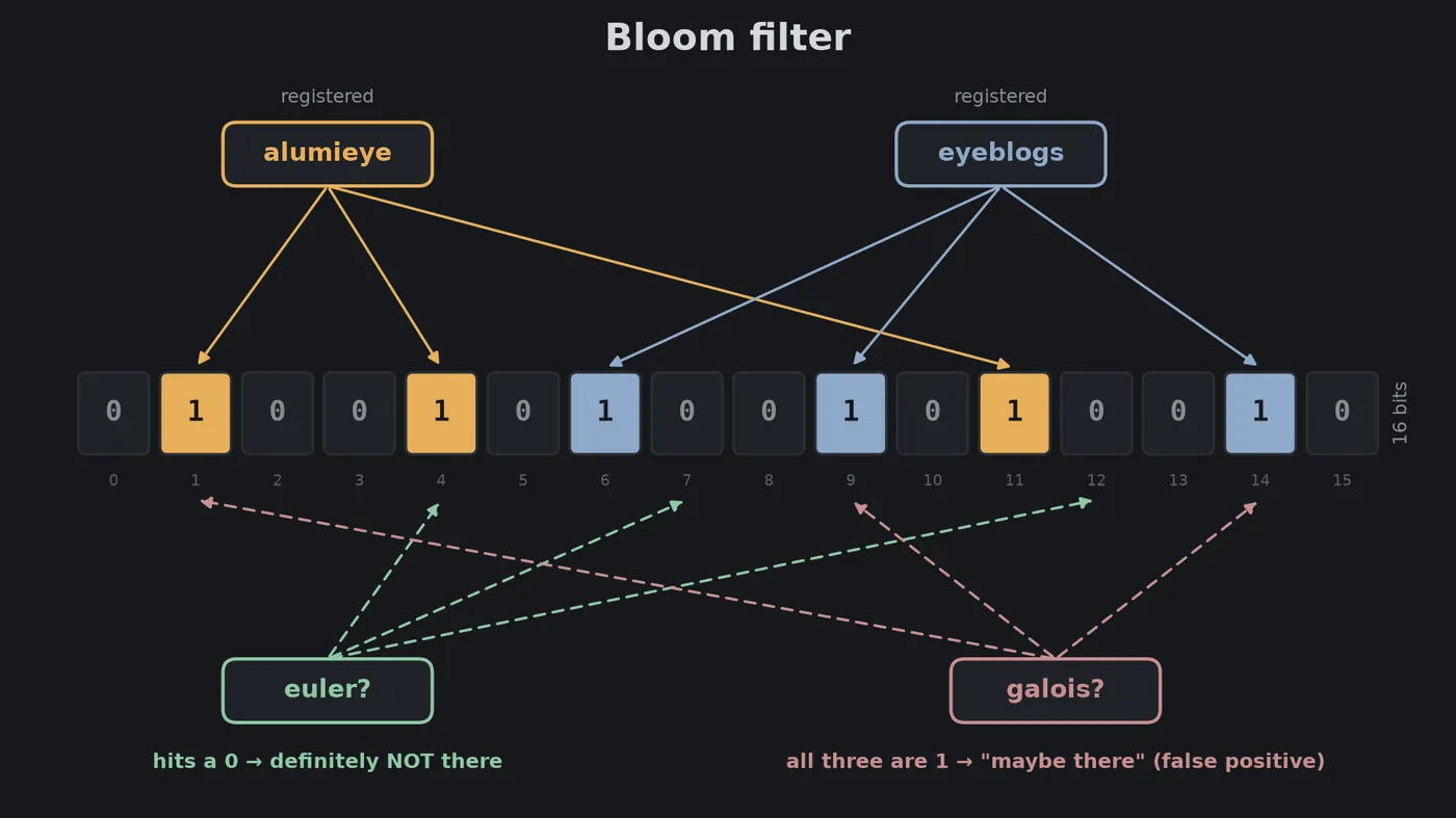
Adding a name: feed it to the grinder and turn on the three switches it points at. Switches that are already on stay on. In the cover image, alumieye turns on cells 1, 4 and 11; eyeblogs turns on cells 6, 9 and 14.
Looking up a name: feed it to the grinder and look at its three switches.
- If at least one switch is off, the name has definitely never been added. Had it been added, all three of its switches would be on. The name
eulerfalls into this case. - If all three are on, the name may have been added. But those three switches may also have been turned on by other names.
galoiswas never added, yet cell 1 was turned on byalumieye, and cells 9 and 14 byeyeblogs. The filter answers wrongly: “maybe”.
That wrong answer is called a false positive. The opposite error, a false negative (the filter says “not there” when the item actually is), never happens, because switches only ever get turned on, never off.
The filter never stores the names themselves. It only stores which switches are on. That is why it is astonishingly small, and also why it can never say “yes” with certainty.
What good is a “maybe”?
The trick is to never use a Bloom filter on its own. It stands guard in front of something slow and expensive, usually a database on disk or a remote service:
- A question comes in. Ask the Bloom filter first, in RAM, in well under a microsecond.
- The filter says “definitely not”: answer right away, nothing more to do.
- The filter says “maybe”: only now ask the database for a definite answer.
With a filter that is wrong 1% of the time, out of every 100 questions about names that do not exist, only about 1 gets sent to the database by mistake. The other 99 are answered in RAM. The error does not make the final answer wrong; it only causes a little extra work. That is why a structure that is “sometimes wrong” ends up inside systems that must be exactly right.
For usernames, Redis, a very popular in-memory database, describes exactly this pattern: if the filter says “no”, create the account straight away; if it says “maybe”, either check the main database or simply ask the user to pick another name[2]. The second option means a free name is occasionally rejected for no reason. For usernames that is acceptable. For a credit card reported as stolen, it is not.
The idea is older than the Internet. In 1970, Burton Bloom wrote the original paper with an example about hyphenation: a dictionary of 500,000 words, 90% of which could be hyphenated with a few simple rules, while the remaining 10% needed a lookup in a table stored on disk, and disk reads were very slow back then. Bloom proposed a small table of bits in memory to tell immediately which words definitely did not need the disk lookup[1]. More than half a century later, systems still use exactly that model: a cheap filter in front, an expensive check behind it.
Where do Bloom filters run today?
Databases: don’t open a file if the key is definitely not there
Write-heavy databases such as Cassandra, RocksDB and HBase store data as many sorted files on disk, as described in the LSM-tree section of the article on binary search and database indexes. Finding one key may mean asking file after file, and every question is a disk read.
So each file comes with a Bloom filter that lives in RAM. Before reading a file, the database asks its filter. “Definitely not” means skip the file, without a single disk read. Cassandra uses a 1% false positive rate by default and lets you tune it per table, trading RAM for accuracy[4].
The biggest win goes to a kind of query that sounds useless: looking for something that does not exist. Without a filter, a query for a missing key is the most expensive query of all, because every file must be opened before you can conclude “not found”. With a filter, it is almost free.
Akamai: three quarters of content is viewed only once
Akamai runs one of the largest content delivery networks (CDNs) in the world: hundreds of thousands of servers placed everywhere, holding copies of web pages, images and videos so users can download them from a nearby machine. Normally, a CDN server keeps a copy of everything it has just served, in case someone asks again.
When Akamai engineers analysed two days of logs from a cluster of 45 servers, they found that among roughly 400 million objects requested, 74% were requested exactly once and never again. They called them “one-hit wonders”. Storing them on disk only wastes space and pushes popular content out[3].
The fix is a “cache on second hit” rule, using a Bloom filter to remember what has been requested before:
- First request for an object: the filter says “not there”. Serve it but do not cache it; just add its name to the filter.
- Second request: the filter says “maybe”. Only now store it on disk.
An experiment on about 47 production servers gave clear results: the share of bytes served from cache rose from about 74% to 83%, and disk writes fell by 44%, from about 10,200 to 5,700 per second[3]. Here a false positive only means an object is occasionally cached one request early. Harmless.
Browsers: checking for phishing without sending every link away
Early versions of Chrome had to check whether each link you opened was on Google’s list of phishing and malware sites. Sending every link to Google would be slow and would leak your browsing. So Chrome kept a Bloom filter of the blocklist on your machine: most links were declared “definitely safe” locally, and only links that came back “maybe” were checked properly with the server.
Around 2011, Chrome replaced the Bloom filter with a different structure called PrefixSet, which takes advantage of the blocklist data being evenly spread out to compress it more tightly[5]. It is a common lesson: a Bloom filter is a good general-purpose answer, but once you understand your data well, there is sometimes a better one.
Medium: ten years of use, then removed
The blogging platform Medium used Bloom filters for its recommendation filters: drop stories you have already read, drop stories from writers you have muted. One filter per user, very fast to query.
In 2025, Medium’s engineering team wrote that they had removed those Bloom filters, replacing them with direct per-user database queries, and that filtering became about 10 times cheaper and easier to maintain[6]. The Bloom filter was not wrong. At Medium’s scale and for their usage, the cost of maintaining millions of filters, keeping them in sync and rebuilding them when needed had grown larger than the benefit. The section “When not to use a Bloom filter” below comes back to this.
How much memory does a Bloom filter need?
A Bloom filter has three numbers:
- : the number of items you plan to add (say, 100 million names).
- : the number of bits in the filter.
- : the number of switches each item turns on, i.e. the number of hash functions.
The easiest way to think about it is in bits per item, . The table below shows how many bits you need to reach a given error rate, with the best number of hash functions at each level[2]:
| False positive rate | Bits per item | Hash functions | Memory for 100 million names |
|---|---|---|---|
| 10% | 4.8 | 3 | 60 MB |
| 1% | 9.6 | 7 | 120 MB |
| 0.1% | 14.4 | 10 | 180 MB |
| 0.01% | 19.2 | 13 | 240 MB |
Two things stand out in this table.
First, the length of the name does not matter. An 8-character username and a 200-character URL cost the same number of bits. For comparison, Redis estimates that an ordinary set costs about 192 bits plus the length of the value itself per item[2]. With 12-character names, 100 million of them in such a set take about 3.6 GB, roughly 30 times the size of a Bloom filter at 1%.
Second, every tenfold drop in the error rate costs only about 4.8 more bits per item. Accuracy is cheap. Going from 1% to 0.01%, i.e. 100 times more accurate, only doubles the size of the filter.
Why the filter “fills up” faster than you think
With 10 bits per name and , each name turns on 7 switches, so 10 million names make 70 million “turn on” moves across 100 million switches. Intuition says about 70% of the switches end up on. In reality only about 50% do, because many moves land on a switch that is already on.
This is the same phenomenon as the birthday paradox (article in Vietnamese): with just 23 people there is already a 50% chance that two share a birthday, because the number of pairs grows faster than the number of people. Collisions arrive sooner than intuition expects. And it turns out the best state for a Bloom filter is exactly when about half of its bits are on: fewer means wasted memory, more means false positives shoot up.
The practical consequence: a filter must be designed for the maximum number of items from day one. Add more than that and the false positive rate does not creep up slowly, it climbs fast. A filter designed for 1% that is stuffed with twice as many items gives false positives about 14% of the time (see Figure 1 at the end of the article).
What a Bloom filter cannot do
It cannot delete. To delete a name, you would have to turn off its switches, but those switches may be shared with other names. Turning them off would create false negatives, the one error a Bloom filter promises never to make. There are two common fixes. A counting Bloom filter replaces each bit with a small counter, costing several times more memory. A cuckoo filter (2014) stores a short “fingerprint” of each item instead of setting bits, supports deletion, and is often more compact than a Bloom filter when you need a very low error rate[7].
It cannot list its contents. The filter does not store names, so you cannot ask “which names are in here?”. To rebuild a bigger filter, you need the original list somewhere.
You must guess its size in advance. As shown above, stuffing in more items than planned makes the error rate shoot up. There are two ways around it. Redis automatically stacks a new filter on top whenever the old one is full, at the cost of queries going through more layers[2]. Akamai uses two filters in rotation: when the primary is full, it becomes the secondary, a fresh empty filter becomes the primary, and the old secondary is thrown away. This keeps the error rate low and automatically “forgets” things nobody has asked for in a while[3].
When not to use a Bloom filter
- The data is small enough to keep in RAM as is. For a few hundred thousand items, an ordinary set is fast enough and exactly right.
- The lookup behind it is already cheap. If the database has a good index and answers in a millisecond, an extra filter layer just adds one more thing to keep in sync. This is roughly Medium’s conclusion.
- False positives are unacceptable and there is no checking layer behind the filter.
- The data changes and gets deleted constantly. A cuckoo filter or another structure fits better.
Bloom filters in system design interviews
From here on we switch to the technical side. Bloom filters come up very often in system design interviews, usually not as the main question but as one piece of the answer. Three classic cases:
- Web crawler: the crawler must remember billions of URLs it has visited so it does not visit them again. A Bloom filter sits in front of the URL store. A false positive means skipping a few pages that were never visited, usually acceptable.
- Checking usernames or coupon codes: exactly the example at the start of this article.
- Recommendation systems: “has this user already seen this item?”. A false positive means occasionally not recommending something you should have.
A good answer usually goes through five steps:
- State what a false positive costs in this problem: one extra database query, a skipped page, or a user wrongly turned away. This is what the interviewer most wants to hear.
- Estimate , pick an error rate , then compute memory: bits, i.e. about 10 bits for 1%. A billion URLs at 1% is about 1.2 GB, which fits in the RAM of one machine.
- Where to put the filter: in the memory of each application server (fastest, but must be kept in sync), or in a shared place like Redis (a single copy, one more network hop). It is the same “where do we count?” question as in the article on rate limiters and the sliding window.
- How to rebuild it when it fills up or when a machine restarts: reload the original list from the database, or periodically save the filter to disk.
- Name an alternative (a cuckoo filter when you need deletion, a plain set when the data is small) to show you know its limits.
The false positive formula
This section uses a little probability. Readers interested only in the applications can skip it.
Assume the hash functions pick switches completely at random. On each “turn on” move, the probability that a particular switch is not picked is . After adding items, each making moves, moves in total, the probability that the switch is still off is:
A name that was never added produces a false positive when all of its switches are on:
The formula shows the tug of war over . Raising means a query must “hit” more switches before it can be fooled, but it also makes the filter light up faster. Taking the derivative shows the balance point is at:
Plugging that back in, at that point : half of the switches are on, exactly as said above. The false positive rate is then , and solving for the bits needed per item:
For , , so you need about bits per item and , matching the table above.
One implementation detail remains: do you really need 7 different hash functions? No. Kirsch and Mitzenmacher proved that two hash values are enough: generate the positions for , and the false positive rate barely changes[8]. The code below uses exactly this trick.
Simulate it yourself
The Python below writes a Bloom filter in about 20 lines, then runs two experiments. Experiment 1 keeps a fixed filter of 100,000 bits (12.5 KB) with , adds up to 20,000 names, and measures the false positive rate on 20,000 names that were never added. Experiment 2 fixes 10 bits per name and varies the number of hash functions from 1 to 15. Every measurement is shown next to the theoretical formula from the previous section. All you need is matplotlib.
import hashlibimport math
import matplotlib.pyplot as plt
plt.rcParams.update({"figure.facecolor": "#16181c", "axes.facecolor": "#16181c", "text.color": "#d4d7dc",                     "axes.edgecolor": "#2a2e35", "xtick.color": "#878d97", "ytick.color": "#878d97", "font.size": 12})

class BloomFilter:    """An array of m bits; each item sets k bits chosen by k hash functions."""
    def __init__(self, m, k):        self.m, self.k = m, k        self.bits = bytearray((m + 7) // 8)
    def _positions(self, item):        # Hash once into two 64-bit numbers h1, h2, then derive k positions h1 + i·h2 (the Kirsch–Mitzenmacher trick).        d = hashlib.blake2b(item.encode(), digest_size=16).digest()        h1, h2 = int.from_bytes(d[:8], "little"), int.from_bytes(d[8:], "little") | 1        return [(h1 + i * h2) % self.m for i in range(self.k)]
    def add(self, item):        for p in self._positions(item):            self.bits[p >> 3] |= 1 << (p & 7)
    def might_contain(self, item):        """False = definitely not there. True = maybe there (check the database)."""        return all(self.bits[p >> 3] >> (p & 7) & 1 for p in self._positions(item))

def theory(m, n, k):    """Theoretical false positive rate: (1 - e^(-kn/m))^k."""    return (1 - math.exp(-k * n / m)) ** k

# Tiny example: 2 registered names.bf = BloomFilter(m=1_000, k=7)for name in ["alumieye", "eyeblogs"]:    bf.add(name)print(bf.might_contain("eyeblogs"), bf.might_contain("euler"))    # True False
# Experiment 1: m = 100,000 bits (12.5 KB), k = 7, add up to 20,000 names.# Measure the false positive rate on 20,000 names that were NEVER added.M, K = 100_000, 7bf = BloomFilter(M, K)tests = [f"chua-co-{i}" for i in range(20_000)]  # "chua-co" = "not added yet" in Vietnamesens, measured = [], []for n in range(1, 20_001):    bf.add(f"user-{n}")    if n % 1_000 == 0:        fp = sum(bf.might_contain(t) for t in tests) / len(tests)        ns.append(n)        measured.append(fp)        if n in (5_000, 10_000, 15_000, 20_000):            print(f"n = {n:>6}  ({M / n:4.1f} bits/name)  measured FP {fp:6.2%}  theory {theory(M, n, K):6.2%}")
# Experiment 2: fix 10 bits per name (m = 100,000, n = 10,000), vary the number of hash functions k.N = 10_000ks, by_k = list(range(1, 16)), []for k in ks:    f = BloomFilter(M, k)    for i in range(N):        f.add(f"user-{i}")    by_k.append(sum(f.might_contain(t) for t in tests) / len(tests))for k in (1, 3, 7, 11, 15):    print(f"k = {k:>2}  measured FP {by_k[k - 1]:6.2%}  theory {theory(M, N, k):6.2%}")print(f"best k in theory: (m/n)·ln 2 = {M / N * math.log(2):.1f}")
# Plotfig, (a1, a2) = plt.subplots(1, 2, figsize=(11, 4.6))grid = range(200, 20_001, 200)a1.plot(list(grid), [100 * theory(M, n, K) for n in grid], color="#8fa9c9", lw=2, label="theory")a1.plot(ns, [100 * x for x in measured], "o", color="#e8b05a", ms=5, label="measured")a1.set_xticks(range(0, 20_001, 5_000))a1.xaxis.set_major_formatter(lambda x, _: f"{x:,.0f}")a1.axvline(M / 9.6, color="#2a2e35", lw=1)a1.text(M / 9.6 + 250, 12, "9.6 bits/name\n→ about 1%", color="#a4a9b2", fontsize=10)a1.set_xlabel("names added (fixed filter of 100,000 bits)", color="#a4a9b2")a1.set_ylabel("false \"maybe there\" rate (%)", color="#a4a9b2")a1.set_title("The fuller it gets, the more it lies", color="#d4d7dc", fontsize=12)
a2.plot(ks, [100 * theory(M, N, k) for k in ks], color="#8fa9c9", lw=2, label="theory")a2.plot(ks, [100 * x for x in by_k], "o", color="#e8b05a", ms=5, label="measured")a2.set_xlabel("number of hash functions k (10 bits per name)", color="#a4a9b2")a2.set_title("Too few or too many hashes both hurt", color="#d4d7dc", fontsize=12)a2.set_yscale("log")a2.yaxis.set_major_formatter(lambda y, _: f"{y:g}")a2.set_ylabel("false positive rate (%, log scale)", color="#a4a9b2")for ax in (a1, a2):    ax.grid(color="#22262c")    ax.legend(frameon=False, labelcolor="#a4a9b2", fontsize=10)fig.tight_layout()fig.savefig("bloom-filter-en.png", dpi=150, bbox_inches="tight")
True Falsen = 5000 (20.0 bits/name) measured FP 0.04% theory 0.02%n = 10000 (10.0 bits/name) measured FP 0.92% theory 0.82%n = 15000 ( 6.7 bits/name) measured FP 4.95% theory 4.91%n = 20000 ( 5.0 bits/name) measured FP 13.95% theory 13.78%k = 1 measured FP 9.88% theory 9.52%k = 3 measured FP 1.55% theory 1.74%k = 7 measured FP 0.92% theory 0.82%k = 11 measured FP 1.16% theory 1.16%k = 15 measured FP 2.38% theory 2.27%best k in theory: (m/n)·ln 2 = 6.9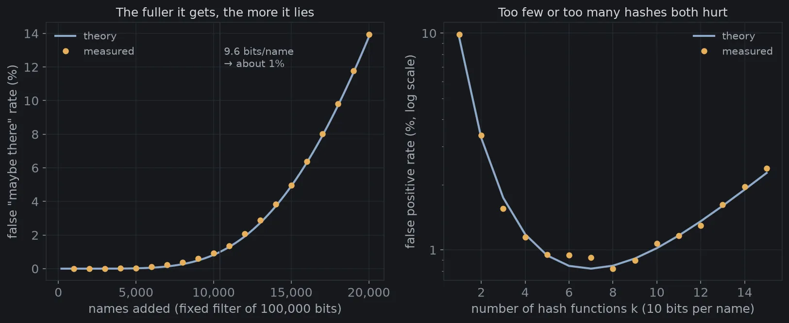
The measured dots track the theory line closely, so the formula above is a trustworthy design tool. Two things to read from the figure:
- Left: at 10,000 names (10 bits per name), the filter gives false positives less than 1% of the time. Stuff in twice as many, 20,000 names, and the error does not double: it grows about 15 times. That is why you design for the maximum number of items from the start.
- Right: the bottom of the curve is quite flat. Every from 5 to 9 gives an error rate around 1%, so in practice you do not need to choose very precisely. The measured dots wobble slightly around the bottom (the lowest one lands at instead of 7), which is just noise from measuring on 20,000 names.
You can change M and K to design a filter for your own problem, then compare the measurements with the table in the “How much memory” section.
Being a little wrong to be a lot faster
The Bloom filter teaches a valuable design habit: when most answers are “no” and the real check is expensive, put a cheap filter in front that can only be wrong in one direction. It does not replace the database. It spares the database from answering questions whose answer is certainly “no”.
The system design side adds a familiar lesson: no data structure is best in every situation. Akamai used a Bloom filter to cut disk writes nearly in half. Chrome and Medium used one for years, then replaced it with something that suited their data better. Knowing where its errors land and what they cost you is the hard part.
Next time a site tells you “this username is already taken” before you have even finished typing, you will know that behind it there may be nothing more than a row of switches, a few of which just lit up because of your name.
Tài liệu tham khảo
- [1]Burton H. Bloom. Space/Time Trade-offs in Hash Coding with Allowable Errors. Communications of the ACM 13(7), 1970.
- [2]Bloom filter (Redis Open Source). Redis Documentation.
- [3]Bruce M. Maggs and Ramesh K. Sitaraman. Algorithmic Nuggets in Content Delivery. ACM SIGCOMM Computer Communication Review 45(3), 2015.
- [4]Bloom Filters. Apache Cassandra Documentation.
- [5]Chromium Safe Browsing: PrefixSet replacing BloomFilter (code review 6286072). Chromium Code Reviews, 2011.
- [6]Engineering stories behind the Medium Daily Digest Algorithm: Part 2. Medium Engineering, 2025.
- [7]Bin Fan, David G. Andersen, Michael Kaminsky and Michael D. Mitzenmacher. Cuckoo Filter: Practically Better Than Bloom. CoNEXT, 2014.
- [8]Adam Kirsch and Michael Mitzenmacher. Less Hashing, Same Performance: Building a Better Bloom Filter. Random Structures & Algorithms 33(2), 2008.