HDD vs SSD: what changes in system design?
HDD vs SSD is about more than speed. Learn how sequential reads, IOPS and latency guide storage choices for databases, video archives and tiered systems.
Mục lục
You copy a movie onto a hard drive. The progress bar moves steadily. But when you open a folder full of small files, the computer keeps pausing. Their combined size might be smaller than the movie, so why does the job take longer?
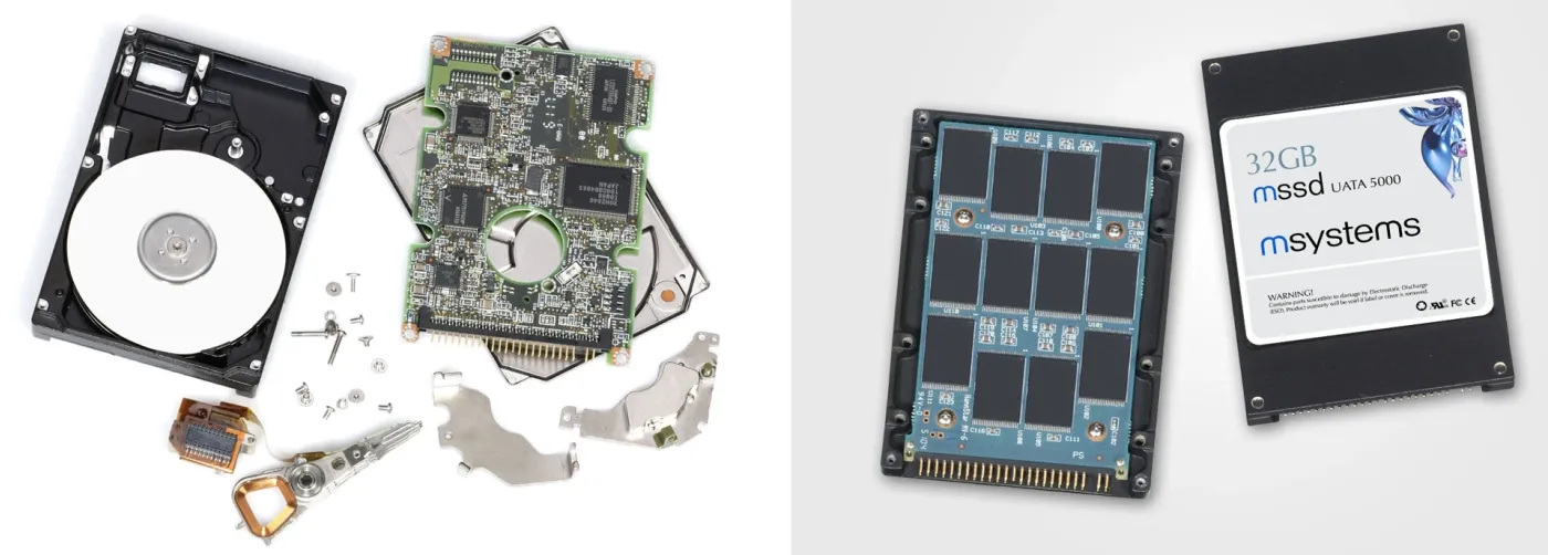
HDD vs SSD is not simply a contest over which drive copies files faster. An HDD reads data using heads and spinning platters, so changing position can involve waiting for mechanical movement. An SSD uses memory chips, without that head-positioning step. SSDs therefore usually have a clear advantage when a system needs many scattered pieces of data. HDDs remain worth considering when you need large capacity at a low cost and mostly read long, continuous stretches[1].
When designing a service, the question goes beyond “how many terabytes do we need?” You also need to know how data will be retrieved, how long users can wait, and what happens when many requests arrive together.
How do HDDs and SSDs work inside?
Imagine a records warehouse with rows of shelves. To retrieve a file, a worker walks to the right shelf and finds its location. If the next customer wants a file at the opposite end, the worker has to move again.
An HDD, short for hard disk drive, involves a similar wait for position. It stores data magnetically on spinning platters. The head assembly must reach the right area, then wait for the required data to rotate underneath. Only then can the drive transfer the data[1].
You can think of a read as having three parts: reaching the right position, waiting for the right section to arrive, and transferring the data. Reading a long stretch spreads that initial waiting cost over many bytes. Jumping between locations repeats it.
An SSD, or solid-state drive, stores data in memory chips, usually NAND flash. Think of a warehouse that selects compartments electronically instead of making a worker walk between them. There is no read head to move into physical position. A controller receives requests and organizes access to the memory chips[1].
That does not mean an SSD returns data instantly. Its controller, memory chips, connection and pending requests can all introduce delays. An SSD removes one major source of HDD waiting, not every source of waiting.
Do not confuse an SSD with RAM, the computer’s working memory. RAM is like the desk where files are laid out for processing; SSDs and HDDs are where files are put away for longer-term storage. Both drive types retain data without power under appropriate operating and storage conditions, but neither replaces RAM’s role.
Why can copying a movie be faster than opening small files?
Sequential reads retrieve adjacent regions of data, like taking a whole stack of files from one shelf. Random reads retrieve scattered locations, like receiving successive requests for files in different aisles.
“Random” describes the access locations here. It does not necessarily mean the program rolls dice. Looking up orders for different customers can produce this pattern even when every query has a deliberate purpose.
A large movie file often creates an opportunity for sequential access. Opening many small files may require retrieving both file-management information and contents from multiple locations. If those locations are scattered, an HDD has to reposition repeatedly. A fragmented large file can also be slow; small files placed close together and read in batches can fare better.
In other words, “one file” and “sequential” do not mean the same thing. The physical layout and the way software issues requests determine the actual work. The operating system may also read ahead or retain previously read data to avoid asking the drive again.
Amazon EBS documentation distinguishes these two workloads. Its SSD-backed volume types target small, frequent operations; its HDD-backed types target large streams and sequential reads and writes[2]. That is a classification of specific AWS services, not a promise that every HDD or SSD has the same performance.
Look beyond the MB/s number on the box
A truck can carry a lot of freight per trip and still take a long time to deliver individual envelopes. Storage also needs to distinguish how much passes through from how long someone waits for one item.
Throughput measures data transferred over a period, often expressed in MB/s or MiB/s. Latency is the time between sending a request and receiving its result. IOPS, input/output operations per second, counts completed delivery trips without telling you how much each trip carries[3].
Suppose a system completes 1,000 reads per second, each exactly 4 KiB. Its throughput is only about 3.91 MiB/s. This is an illustrative calculation: multiply the operation count by the size per operation, then convert units. It is not a measurement of a drive model.
If every read were 1 MiB and the system still sustained 1,000 reads per second, throughput would be 1,000 MiB/s. But that “if” matters: drives and connections have their own limits. Increasing the operation size may reduce operations per second. You cannot combine the maximum IOPS from one test with the maximum MB/s from another and treat them as a single operating point.
Here, a KiB is 1,024 bytes, and a MiB is 1,024 KiB. The decimal unit MB is 1,000,000 bytes. Like two different ways of packing boxes, the units need to match before comparing their numbers.
How many requests are waiting together?
Queue depth (QD) describes how many requests remain outstanding at a given moment. QD of 1 is like a customer who orders the next dish only after receiving the previous one. A higher QD is like several order tickets waiting in a kitchen.
An SSD can use concurrent requests to work across different parts of its memory. An HDD may reorder some requests to reduce movement. But adding requests does not create unlimited resources: eventually the queue grows and customers wait longer[3].
A high IOPS figure therefore needs context: operation size, read/write mix and queue depth. For a checkout page, the wait for an individual request can matter more than an impressive aggregate benchmark figure.
Why can the same 256 MiB take different amounts of time?
Let us build an imaginary warehouse with two drive types. Its HDD needs 8 milliseconds of setup whenever it moves to a new region, then transfers at 180 MiB/s. Its SSD needs 0.1 milliseconds of setup per operation, then transfers at 500 MiB/s. All these parameters are chosen for illustration, not to represent a particular product.
We read 256 MiB in total through consecutive requests, without cached data or request merging. Each small request accesses a new region. The final case reads one continuous stretch and pays the setup cost just once. The code near the end produces these results:
| Reading pattern in the model | Operations | HDD | SSD |
|---|---|---|---|
| Scattered 4 KiB reads | 65,536 | 525.71 seconds | 7.07 seconds |
| Scattered 64 KiB reads | 4,096 | 34.19 seconds | 0.92 seconds |
| Scattered 1 MiB reads | 256 | 3.47 seconds | 0.54 seconds |
| One continuous 256 MiB stretch | 1 | 1.43 seconds | 0.51 seconds |
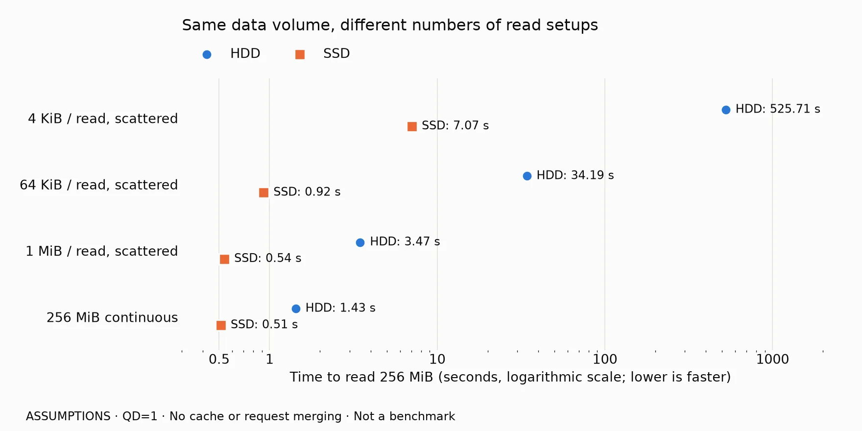
With 4 KiB reads, the model’s HDD spends most of its time on 65,536 setup steps. With one long stretch, that part almost disappears. The SSD remains faster, but the gap depends on the access pattern rather than a fixed multiplier.
The model deliberately leaves out read-ahead, caching, parallelism, actual disk positions and filesystem overhead. Its last row does not claim that the operating system issues a single 256 MiB command. It represents an ideal continuous stream, not a real device’s command splitting.
The lesson is that batching data helps only when it actually reduces searching and waiting. Packing many files into one large file, then still jumping between scattered locations, does not necessarily deliver the same benefit.
Does a database need capacity or fast lookups?
Suppose you open your order history. The database finds your customer ID in a directory, then retrieves the corresponding data pages. An index is like the warehouse catalog: instead of reading through the whole collection, it points toward locations that may contain the desired records.
But the catalog and the records can occupy different places. A query returning little text may still need to read many pages from storage. The article on binary search and database page reads explains why reducing reads often matters more than saving a few comparisons.
An SSD is usually a reasonable starting point for frequently queried data that needs short response times. Still, replacing a drive does not fix a query that searches the entire warehouse for one order. If the required data is already in RAM, a faster drive may make little difference to that query.
A cache keeps copies for reuse, like a stack of records already sitting on the desk. It reduces trips to the warehouse. But after startup, or when a requested record is absent, the system still has to access storage. Measure both warm-cache and empty-cache conditions. The story of a changed profile picture that still looks old explores the benefits and costs of those copies.
Why do databases write to a log first?
When updating files on several shelves, there is a way to avoid immediately running around the warehouse: record the changes in order in a notebook, then update the shelves later.
That is the intuition behind a write-ahead log (WAL). PostgreSQL requires the corresponding log information to reach durable storage before changed data pages are written. With a durable-commit configuration, a transaction can be acknowledged once the necessary log records are durable. Data pages can be written later and recovered from the log[4].
“Durable” means more than placing data in the operating system’s RAM. It is like putting the notebook in storage that survives the failures covered by the system’s guarantees, rather than leaving a note on the desk. Operations that request data be flushed to storage, such as fsync, directly affect how long confirmation takes.
Appending records helps reduce HDD movement. On SSDs, reducing synchronization calls and batching work can still help. But WAL does not turn an entire database into one sequential stream: record reads and later page updates still exist. This also makes the logbook approach behind Kafka useful to understand, though systems that use logs do not all share the same architecture.
What are an SSD’s drawbacks besides price?
NAND does not behave like paper on which you can erase any single letter at will. It programs pages but erases larger blocks. For an update, the controller generally writes the new data elsewhere and marks the old copy invalid[6].
When reclaiming space, it may have to move still-valid pages out of a block before erasing the whole block. Garbage collection is like clearing a shelf: the valuable records must be moved elsewhere before the old section can be discarded.
These internal copies cause write amplification: an application submits some amount of data, but the memory chips perform more writing behind the scenes. Like updating one file while also having to relocate the surrounding stack, the internal work exceeds the original request[6].
Flash chips also have finite write/erase endurance. TBW, terabytes written, is a cumulative-write rating used in endurance specifications. Read the definition and warranty conditions of the particular drive. It resembles the mileage allowance in a vehicle warranty, not a promise that the device will fail the instant it reaches that figure[1].
Write-heavy systems therefore need to consider sustained speed after the initial short burst, free space, write endurance and power-loss behavior. Having no moving parts does not eliminate the possibility of data loss. Both HDDs and SSDs need a backup plan and tested recovery procedures.
Are SATA and NVMe two kinds of memory?
No. SATA and NVMe describe ways of communicating with storage devices, like the transport routes into a warehouse rather than what is stored inside. An SSD can use SATA; NVMe commonly runs over PCIe to exploit a connection and processing model suited to flash memory[5].
M.2 is instead a common physical form factor and connection format, like a doorway’s dimensions and connector shape[5]. Some M.2 SSDs use SATA, while others use NVMe. Seeing a small stick-shaped drive does not establish its speed or compatibility.
In system design, the interface name is only part of the picture. An SSD with a fast connection can still be limited by its access pattern, temperature, controller or pending work.
Should you choose HDDs, SSDs or both?
Return to the records warehouse. Frequently requested files belong near the service counter. Older boxes can sit farther away, provided retrieval still meets people’s needs.
Tiered storage uses the same idea: place data in layers with different costs and service characteristics. “Hot” data is frequently used, such as orders currently being processed. “Cold” data is rarely requested, such as source footage from a finished video that is only occasionally reopened. Neither word refers to drive temperature.
| Main workload | A starting point to consider | What to check |
|---|---|---|
| Transaction lookups, many small reads | SSD | Latency under concurrent load; whether data is already in RAM |
| Interactive search across scattered locations | SSD | Storage regions accessed per request |
| Source-video archive, mostly whole large files | HDD or a low-cost capacity tier | Aggregate throughput with concurrent readers |
| Continuously written and processed logs | Depends on workload; SSD or HDD | Whether access is genuinely sequential; required durable-acknowledgment latency |
| Long-term storage, rare access | An appropriate low-cost tier | Retrieval time, access charges and tested recovery |
These are starting points, not rigid rules. A video archive with thousands of people seeking different clips presents a different workload from one person copying whole files. Multiple logging streams also do not necessarily become one sequential stream at the final device.
Cost should reflect the service delivered, not just purchased capacity. HDDs may cost less per terabyte, but needing many drives to meet lookup demand can erode that saving. An SSD that costs more per terabyte may still make sense for a small, frequently accessed dataset[1].
For cloud storage, read the service limits: capacity, IOPS, throughput, latency and host-side constraints. EBS documentation notes that both instance configuration and operation characteristics can limit performance[2]. An “SSD” label does not guarantee that an application can exploit the underlying chips’ speed.
Before deciding, identify typical read/write sizes, concurrency and the share of scattered access. Then test a realistic workload long enough to see steady-state behavior, not just the initial burst. Record the waiting times of slower requests too. For example, p99 is a latency threshold at or below which 99% of operations complete. It is like looking near the slow end of a restaurant queue instead of only averaging everybody’s service time.
Try modeling the cost of finding each read location
This Python code creates the exact chart and table above. Run it from the project directory with matplotlib available. It only performs calculations; it does not benchmark the drive or overwrite existing drive data. There is no randomness, so repeated runs produce the same results.
The model adds the number of operations multiplied by setup cost to the total data volume divided by transfer rate. Change the assumptions in drives, or the values in sizes, to explore how batching changes the result.
from pathlib import Path
import matplotlibmatplotlib.use("Agg")import matplotlib.pyplot as pltfrom matplotlib.ticker import FuncFormatter
# Illustrative model; no real storage reads or benchmark writes.TOTAL = 256 * 1024**2sizes = [4 * 1024, 64 * 1024, 1024**2, TOTAL]labels = ["4 KiB / read, scattered", "64 KiB / read, scattered",          "1 MiB / read, scattered", "256 MiB continuous"]drives = {"HDD": (0.008, 180 * 1024**2),          "SSD": (0.0001, 500 * 1024**2)}colors = ["#2a78d6", "#eb6834"]surface, ink, grid = "#fcfcfb", "#0b0b0b", "#e1e0d9"plt.rcParams.update({"font.family": "DejaVu Sans", "font.size": 12,                     "text.color": ink, "axes.labelcolor": ink,                     "xtick.color": ink, "ytick.color": ink})fig, ax = plt.subplots(figsize=(11, 5.5), facecolor=surface)ax.set_facecolor(surface)for i, (name, (delay, rate)) in enumerate(drives.items()):    # QD=1: finish one request before issuing the next.    times = [(TOTAL // size) * delay + TOTAL / rate for size in sizes]    ys = [j + (i - 0.5) * 0.25 for j in range(len(sizes))]    ax.scatter(times, ys, s=90, marker=["o", "s"][i], color=colors[i],               edgecolor=surface, linewidth=1.5, label=name, zorder=3)    for t, y in zip(times, ys):        text = f"{name}: {t:.2f} s"        ax.annotate(text, (t, y), xytext=(9, 0),                    textcoords="offset points", va="center", fontsize=11)    print(name, ", ".join(f"{t:.4f} s" for t in times))ax.set_xscale("log")ax.set_xlim(0.3, 2500)ax.set_xticks([0.5, 1, 10, 100, 1000])ax.xaxis.set_major_formatter(FuncFormatter(lambda x, _: f"{x:g}"))ax.set_yticks(range(len(labels)), labels)ax.set_ylim(3.5, -0.6)ax.set_xlabel("Time to read 256 MiB (seconds, logarithmic scale; lower is faster)")ax.set_title("Same data volume, different numbers of read setups", loc="left", pad=44)ax.grid(axis="x", color=grid, linewidth=0.7)ax.tick_params(axis="both", length=0)for spine in ax.spines.values():    spine.set_visible(False)ax.legend(loc="lower left", bbox_to_anchor=(0, 1.02), ncol=2, frameon=False)fig.text(0.03, 0.025, "ASSUMPTIONS · QD=1 · No cache or request merging · Not a benchmark", fontsize=11)fig.tight_layout(rect=(0.01, 0.075, 0.99, 0.99))out = Path("images/hdd-vs-ssd/kich-thuoc-luot-doc-en.png")out.parent.mkdir(parents=True, exist_ok=True)fig.savefig(out, dpi=160, facecolor=surface)plt.close(fig)
Removing the sequential wait requires another model, not simply dividing all times by the number of concurrent requests. Devices have their own limits, and simultaneous work also creates queues. This calculation separates positioning overhead from data transfer; it does not predict your computer’s performance.
Back to the movie and the folder full of files
The movie can copy quickly because it lets the drive perform one long task with fewer stops to find somewhere else. A folder of small files may repeat the setup work even when it contains fewer bytes. SSDs greatly reduce mechanical waiting, while better data organization reduces the number of retrieval trips.
In system design, you are not merely buying a warehouse large enough to hold everything. You are designing how to serve people who keep arriving to request records. Choosing an HDD or SSD begins by looking at what they request, in what order, and how long they can stand waiting.
Cover photo: Rochellesinger / Wikimedia Commons, licensed under CC BY-SA 2.5. Resized and converted to WebP; the converted image is shared under the same license.
Create free geometry illustrations for students and teachers: EyeViz.
Tài liệu tham khảo
- [1]Hard disk drive versus solid-state drive. IBM Think.
- [2]Amazon EBS volume types. Amazon Web Services.
- [3]Amazon EBS I/O characteristics and monitoring. Amazon Web Services.
- [4]Write-Ahead Logging (WAL). PostgreSQL Documentation.
- [5]Solid-state drives (SSDs). IBM Think.
- [6]Write amplification. Wikipedia.