Gauss and the lost asteroid: how least squares was born
In 1801 a new body vanished into the Sun's glare. A 24-year-old found it again with pen and paper, using an idea that now runs in GPS and machine learning.
Mục lục
A star that would not stay still
On the first night of the 19th century, 1 January 1801, the astronomer Giuseppe Piazzi at the Palermo observatory in Sicily was mapping stars. He recorded the position of a faint point of light in the constellation Taurus. The next night, it had moved a little. The night after that, it moved again.
Stars do not move like that. Piazzi had found a new body in the Solar System. He named it Ceres, after the Roman goddess of agriculture, the patron of Sicily.
Piazzi tracked Ceres 24 times over 41 days. On 11 February he fell ill and had to stop observing. By the time he recovered, Ceres had drifted into the part of the sky near the Sun and was lost in daylight[2]. It would be invisible for months.
The problem was that in those 41 days Ceres traced only a very short arc across the sky, less than ten degrees. From such a tiny piece of curve, someone had to work out an entire orbit around the Sun, then compute where, months later, it would reappear among a sky full of stars. Nobody knew how to do that. European astronomers made different predictions, and the sky where they pointed stayed empty.
The newly discovered body was at risk of being lost forever.
At the end of 1801, a 24-year-old in Brunswick, Germany, who had never worked as a professional astronomer, sent out a prediction completely different from everyone else’s. And Ceres appeared almost exactly where he pointed.
This is the third article in a series on mathematicians. By the end you will see what idea found Ceres again, and why it runs in your phone every time you open a map.
The celestial police
Piazzi’s discovery did not come out of nowhere. Since the late 18th century, many astronomers believed there had to be a planet between the orbits of Mars and Jupiter. The gap between those two orbits was unusually wide, and a numerical rule then widely trusted, the Titius–Bode law, “predicted” a planet in exactly that spot.
In 1800 the astronomer Franz Xaver von Zach gathered a group of colleagues across Europe and divided the sky into zones so each could search one part. They called themselves the “celestial police”. Ironically, Piazzi found Ceres by chance before his invitation to join had even reached him.
Ceres sat at exactly the distance everyone expected. Today we know it is not a major planet but the largest body in the asteroid belt, about 940 km across, classified since 2006 as a dwarf planet. But in 1801 it was the “missing planet”, and all of European astronomy wanted it back.
The young man from Brunswick
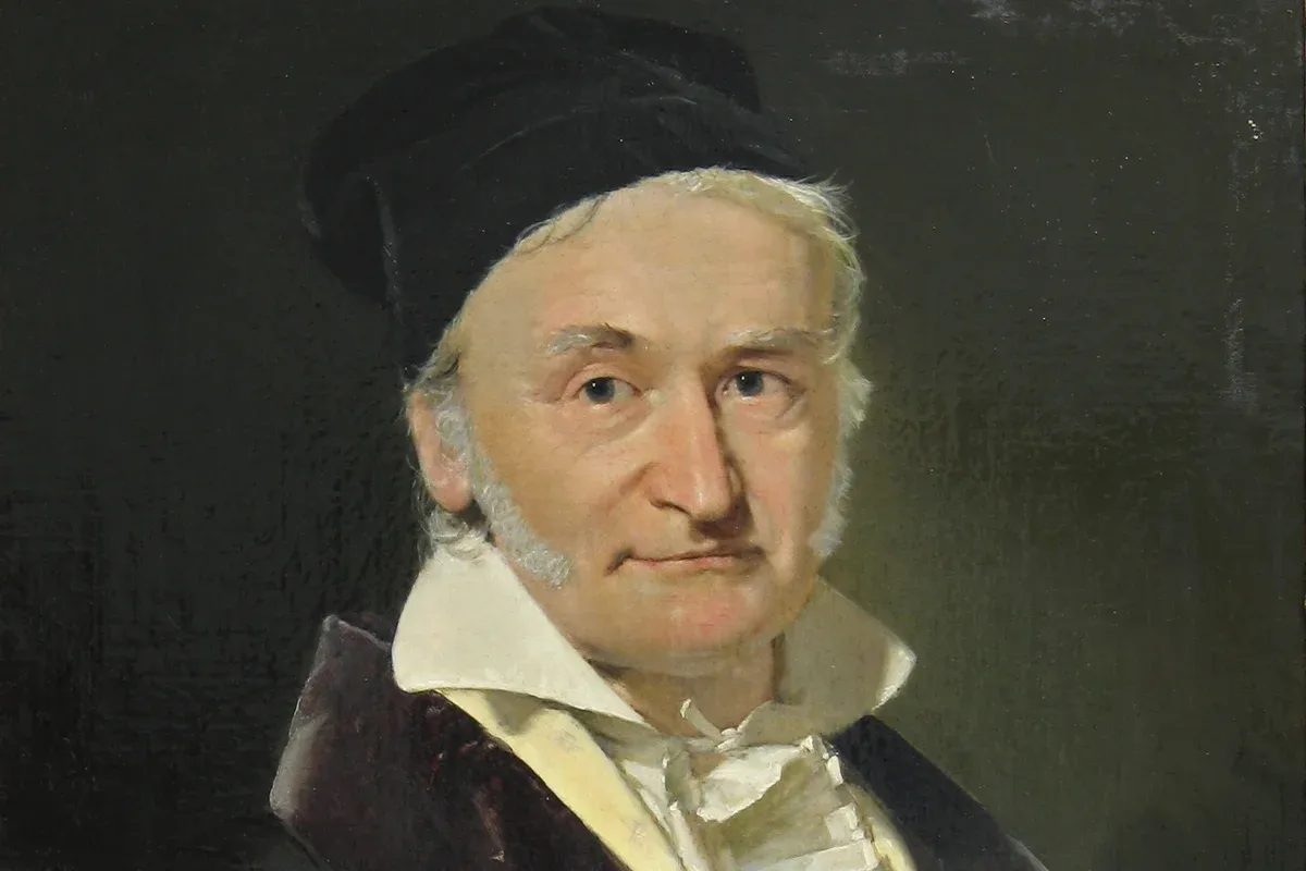
Carl Friedrich Gauss was born in 1777 into a poor family in Brunswick. His father was a bricklayer and gardener. Gauss’s mathematical talent showed so early that the Duke of Brunswick paid for his university studies.
In 1796, not yet 19, Gauss proved that a regular 17-sided polygon can be constructed with only a ruler and compass. The question had stood open since ancient Greece, for more than two thousand years. He was so pleased that he chose mathematics over classical languages, and later wanted the 17-gon carved on his tombstone. In 1801, the same year Ceres disappeared, he published Disquisitiones Arithmeticae, the book that laid the foundations of modern number theory[1].
So in 1801 Gauss was a young number theorist, not an astronomer. But the Ceres problem attracted him for one reason: it was a problem of computation, and a method was missing. He started that autumn, when Piazzi’s observations were published. Within a few weeks he had an orbit.
Two ideas
Gauss’s solution had two parts. The first was a new method for determining the orbit of a body from just three observations, based on Kepler’s laws: every planet moves on an ellipse with the Sun at one focus, following exact rules about its speed. That part was a feat of computation, full of trigonometric manipulation, but it is not the most famous part.
The second part is the question every scientist working with measurements must face: there are 24 observations, but every one of them has errors. The telescope shakes a little, the eye misreads a scale a little, the air blurs the star a little. No orbit passes exactly through all 24 points. So which orbit should you choose?
Using only three points wastes the other 21 observations, and if one of those three happens to be badly off, the whole prediction goes off with it. Simply averaging doesn’t work either, because it is unclear what to average: the observations are at different times and different positions.
Gauss answered with a principle: choose the orbit that makes the sum of the squared deviations between the orbit and the observations as small as possible. If observation deviates from the orbit by , find the orbit that makes
as small as it can be. This principle is called the method of least squares.
Why squares?
Why square the deviations, instead of adding them up directly or taking absolute values?
The first reason is sign. A deviation can be negative or positive: the observation lies inside or outside the orbit. Added directly, a deviation of +5 and one of −5 cancel to 0, as if the orbit fit perfectly. Squaring makes every deviation positive.
The second reason is punishing large errors. A deviation of 2 counts as 4, a deviation of 10 counts as 100. The method therefore strongly dislikes orbits that leave a few points far away, and prefers orbits that are a little off for everyone.
The third reason is ease of computation, the most practical one. With squares, the “find the minimum” problem turns into solving a system of linear equations, something that in 1801 could be done by hand, if slowly.
Gauss went further. In his 1809 book he showed that if measurement errors follow a certain bell-shaped distribution, least squares gives the most probable answer[3]. That bell-shaped distribution is now called the normal distribution, or the Gaussian distribution.
Ceres reappears
Gauss’s computations were published by von Zach at the end of 1801. They differed sharply from the other predictions. Then, in the last nights of the year, once Ceres had left the Sun’s glare, von Zach pointed his telescope where Gauss said, and saw it. Soon afterwards, the astronomer Heinrich Olbers in Bremen observed it too. Ceres was less than one degree from where Gauss had predicted[2].
The 24-year-old became famous across Europe overnight. In 1807 Gauss became director of the Göttingen observatory, a post he held for nearly fifty years, until the end of his life.
Who thought of it first?
Gauss did not publish his method right away. He made a habit of printing only work polished beyond any objection. His motto was “few, but ripe”.
In 1805, the French mathematician Adrien-Marie Legendre published a book on the orbits of comets, with a short appendix that clearly set out the method of least squares, under the name we still use today[4]. Four years later, in Theoria motus (1809), Gauss presented the same method and wrote that he had been using it since 1795.
Legendre was annoyed. He wrote to Gauss that one should not claim priority without a publication to prove it, and later objected publicly. Gauss never produced written proof. Only a few colleagues, Olbers among them, confirmed that Gauss had shown them the method before 1805. Historians of statistics today generally believe Gauss did use the idea early. But Legendre was the first to publish it clearly, and Gauss was the first to put it on a theoretical foundation in probability[5].
A small simulation: why more observations are better
To see the value of the idea, let’s build a simplified simulation. An asteroid moves on a circular orbit around the Sun, radius 2.77 astronomical units (AU, the Earth–Sun distance), like Ceres. We observe it 24 times over 41 days, each measurement off by a little random error. Then we predict its position 300 days later.
Two ways to predict:
- Use only 3 observations: the first, the middle and the last.
- Use all 24 observations and choose the orbit by the least-squares principle.
Each method is repeated 500 times, each time with a fresh set of measurement errors:
| Method | Mean error | 95% of cases below |
|---|---|---|
| 3 observations | 0.28 AU | 0.66 AU |
| 24 observations, least squares | 0.13 AU | 0.32 AU |
Using all 24 observations Gauss’s way cuts the error to about half. In the sky, that is the difference between finding the body right in the telescope’s field of view and having to search an area twice as wide.
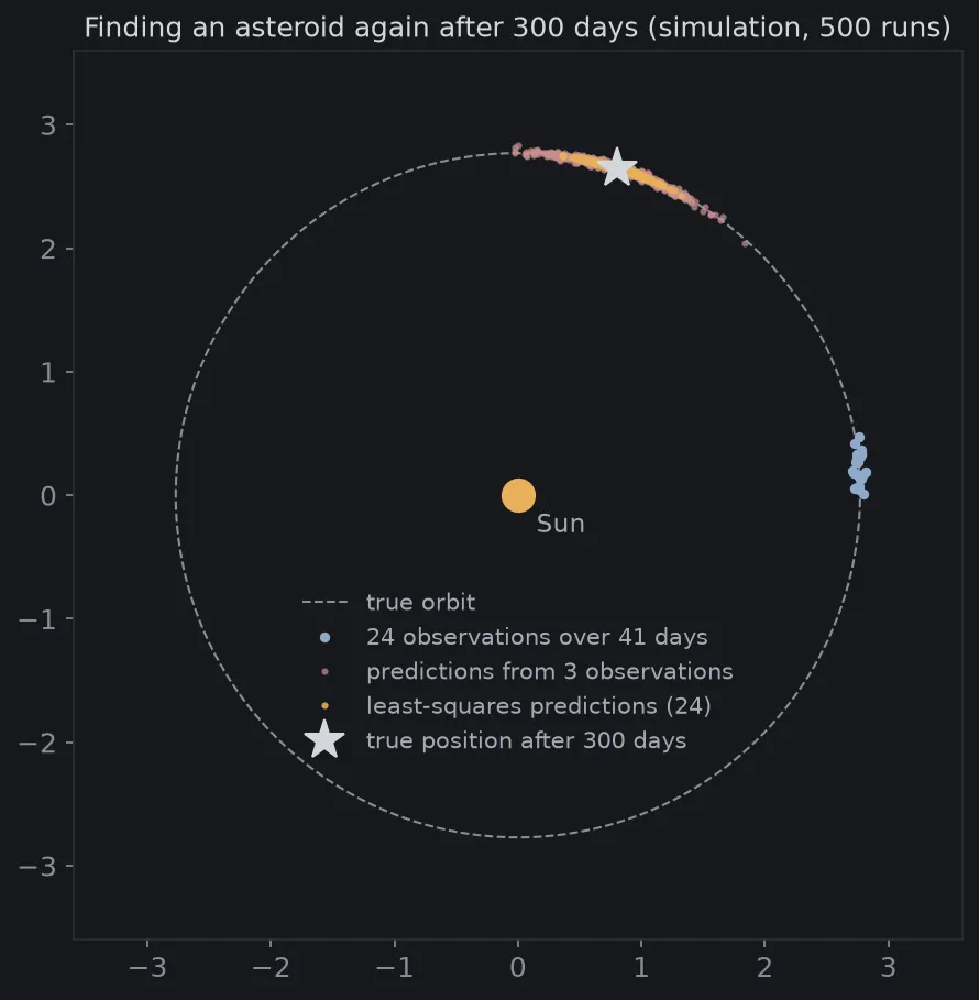
This simulation is far simpler than the real problem. Gauss had to work with elliptical orbits, and with observations that only gave a direction as seen from the Earth, itself in motion, not a distance. But the core idea is the same: don’t trust a few numbers, let every observation “vote”, and let random errors cancel each other out.
Where is the idea today?
The blue dot on the map
When you open a map on your phone, the blue dot showing your position is computed from the signals of navigation satellites. Each satellite tells the phone how far away it is, but that distance always has errors: the signal is slowed by the atmosphere and bounced off tall buildings. In theory, four satellites are enough to fix position and time. But a phone usually “sees” more than that. It does not throw any away; it finds the position that makes the sum of the squared deviations as small as possible, in exactly the spirit of Gauss and his 24 observations of Ceres.
Watching for near-Earth asteroids
The problem of 1801 is still being solved every day, on a much larger scale. Asteroid tracking centers compute the orbits of tens of thousands of near-Earth objects from observations sent in from all over the world, using modern versions of least squares.
The story of the asteroid Apophis shows this most clearly. When it was discovered in 2004, there were few observations, and its computed orbit was very uncertain. For a few days at the end of that year, the chance of it hitting the Earth in 2029 was estimated at a few percent, an unprecedented number. Then astronomers found earlier images of it that nobody had noticed. With more observations the uncertainty shrank, and an impact in 2029 was ruled out completely. In 2029 Apophis will pass very close, but safely. Just like the simulation above: the more observations, the tighter the cloud of predictions.
The best-fitting line
Least squares has a name more familiar to students: linear regression. When someone draws a straight line “through the middle” of a cloud of data points, say height against weight, or electricity use against outdoor temperature, they are almost certainly using the method of Gauss and Legendre.
Many modern machine learning models are trained in the same spirit: choose the parameters that make the sum of squared errors between predictions and data as small as possible. The term squared loss that AI practitioners use every day is exactly the sum of squared deviations of 1801, only now with millions of parameters instead of a few numbers describing an orbit.
Find the asteroid again yourself
The Python below runs the simulation above and draws Figure 1. You need numpy and matplotlib. The model is deliberately simplified: a circular orbit with the Sun at the center, and positions measured directly. Gauss’s real problem was much harder.
import matplotlib.pyplot as pltimport numpy as np
plt.rcParams.update({"figure.facecolor": "#16181c", "axes.facecolor": "#16181c", "text.color": "#d4d7dc",                     "axes.edgecolor": "#2a2e35", "xtick.color": "#878d97", "ytick.color": "#878d97", "font.size": 12})rng = np.random.default_rng(1801)  # Fixed seed: every run gives the same result.
# Simplified simulation: a circular orbit around the Sun, radius 2.77 AU, period 4.6 years.R, PERIOD = 2.77, 4.6 * 365.25OMEGA = 2 * np.pi / PERIOD                 # true angular speed, radians per daydays = np.linspace(0, 41, 24)              # 24 observations over 41 daysLATER = 41 + 300                           # the object must be found again 300 days after the last observationNOISE = 0.03                               # each measurement is off by a few hundredths of an AU

def observe():    """Measured position (x, y): the true position plus random measurement error."""    angle = OMEGA * days    xy = np.column_stack([R * np.cos(angle), R * np.sin(angle)])    return xy + rng.normal(0, NOISE, xy.shape)

def fit(xy, idx):    """Least squares over observations idx: radius r, starting angle, angular speed."""    r = np.hypot(xy[idx, 0], xy[idx, 1]).mean()    ang = np.arctan2(xy[idx, 1], xy[idx, 0])    speed, start = np.polyfit(days[idx], ang, 1)   # best-fitting straight line of angle against time    return r, start, speed

def predict(params, day):    r, start, speed = params    return np.array([r * np.cos(start + speed * day), r * np.sin(start + speed * day)])

truth = predict((R, 0.0, OMEGA), LATER)three, all24 = [], []for _ in range(500):                               # repeat 500 times, each with fresh measurement errors    xy = observe()    three.append(predict(fit(xy, [0, 12, 23]), LATER))     # only 3 observations    all24.append(predict(fit(xy, list(range(24))), LATER)) # all 24 observationsthree, all24 = np.array(three), np.array(all24)for name, p in [("3 obs", three), ("24 obs", all24)]:    err = np.linalg.norm(p - truth, axis=1)    print(f"{name:<7} mean error {err.mean():.3f} AU, 95% of cases below {np.quantile(err, 0.95):.3f} AU")
# Plot: the orbit, the observed arc, and the two "clouds" of predictions around the true position.fig, ax = plt.subplots(figsize=(7.5, 7))t = np.linspace(0, 2 * np.pi, 400)ax.plot(R * np.cos(t), R * np.sin(t), color="#878d97", lw=1, ls="--", label="true orbit")xy = observe()ax.plot(xy[:, 0], xy[:, 1], ".", color="#8fa9c9", ms=7, label="24 observations over 41 days")ax.plot(three[:, 0], three[:, 1], ".", color="#c98f8f", ms=4, alpha=0.6, label="predictions from 3 observations")ax.plot(all24[:, 0], all24[:, 1], ".", color="#e8b05a", ms=4, alpha=0.8, label="least-squares predictions (24)")ax.plot(*truth, "*", color="#d4d7dc", ms=18, label="true position after 300 days")ax.plot(0, 0, "o", color="#e8b05a", ms=14)ax.text(0.15, -0.3, "Sun", color="#a4a9b2", fontsize=11)ax.set_aspect("equal")ax.set_xlim(-3.6, 3.6)ax.set_ylim(-3.6, 3.6)ax.legend(loc="center", bbox_to_anchor=(0.5, 0.3), frameon=False, labelcolor="#a4a9b2", fontsize=10)ax.set_title("Finding an asteroid again after 300 days (simulation, 500 runs)", color="#d4d7dc", fontsize=12)fig.savefig("ceres-en.png", dpi=150, bbox_inches="tight")
3 obs mean error 0.276 AU, 95% of cases below 0.658 AU24 obs mean error 0.133 AU, 95% of cases below 0.319 AUThe np.polyfit function is least squares itself: it finds the straight line (angle against time) with the smallest sum of squared deviations from the observations. Try raising NOISE or shortening the observation period to see how hard Gauss’s problem becomes when the observed arc is too short.
Back to the last night of 1801
Ceres was not lost. It was found again because one person refused to throw away most of the data, and also refused to trust any single number blindly. Gauss treated each observation as a testimony that might be slightly wrong, then looked for the story that best fit all the testimonies at once.
Two hundred years later, that way of thinking is everywhere: in the blue dot on the map, in the calculations that watch over near-Earth asteroids, and in millions of machine learning models trained every day. In 2015, NASA’s Dawn spacecraft entered orbit around Ceres and photographed its surface from a few hundred kilometers away. The faint point of light Piazzi nearly lost is now a world with mountains, impact craters and bright, glittering patches of salt.
The previous article in this series is about Euler and the seven bridges of Königsberg. The next is about Galois, the 20-year-old who scribbled down his mathematical ideas on the night before a duel.
Tài liệu tham khảo
- [1]J. J. O'Connor and E. F. Robertson. Carl Friedrich Gauss (1777–1855), biography. MacTutor History of Mathematics, University of St Andrews.
- [2]Ceres (dwarf planet). Wikipedia.
- [3]Carl Friedrich Gauss. Theoria motus corporum coelestium in sectionibus conicis solem ambientium. Perthes et Besser, Hamburg, 1809.
- [4]Adrien-Marie Legendre. Nouvelles méthodes pour la détermination des orbites des comètes. Firmin Didot, Paris, 1805.
- [5]Stephen M. Stigler. Gauss and the Invention of Least Squares. The Annals of Statistics, 9(3), 465–474, 1981.