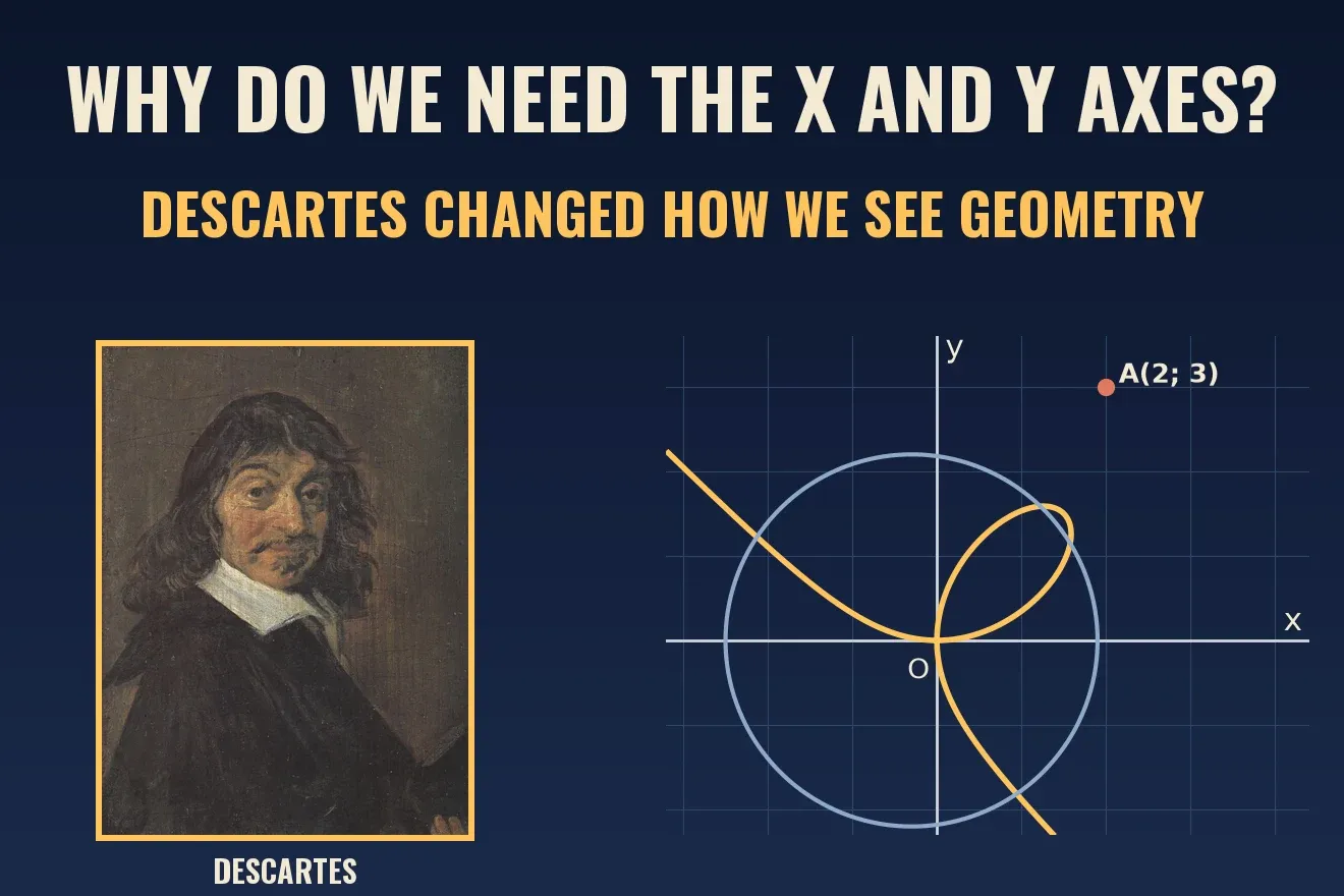
Why do we need the x and y axes? Descartes changed how we see geometry
Why do we need the x and y axes? From the spider-on-the-ceiling legend to the Pappus problem, how Descartes turned geometry into calculation.
Mục lục
Why do we need the x and y axes?
In 7th grade you draw two perpendicular lines, write an O where they cross, an x and a y at the ends, then mark a point and write A(2; 3). Two numbers, one point. It sounds simple, but it is one of the heavyweight ideas of mathematics: it turns a drawing into a calculation.
The short answer: we need coordinate axes because two numbers pin down a point, so a drawing can be written as an equation and solved by calculation. The person who laid the foundation for that idea is René Descartes, the French mathematician and philosopher. His name is inside the word “Cartesian” in “Cartesian coordinate system”[2]. But the story is not as simple as one man drawing two lines. The perpendicular coordinate system from the classroom does not appear in his book. It took shape afterward[2][4].
This article focuses on how he came up with the idea. We will look at the famous anecdote of the spider on the ceiling and ask how much of it holds up, then turn to the documented part: an ancient problem of Pappus. After that comes what really changed in how people see geometry, and where the idea is running today: from rockets to GPS, 3D graphics and artificial intelligence.
What are the axes for?
The idea sits right inside the notation A(2; 3): two numbers pin down a point. The first number is the position across, the second is the position up, both measured from the origin O.
You use this idea outside the classroom without noticing. On a chess board, the square e4 is a pair made of a letter and a number. At a cinema, a ticket says “row F, seat 12”: two pieces of information point to exactly one seat. On a phone screen, every lit dot has two coordinates.
With this naming, a drawing becomes a list of pairs of numbers. A line is the set of all points that satisfy a relation between two numbers. A circle centered at O with radius 5 is every point where . Geometry can now be solved by calculation. That is the step Descartes took, and the question is how he came to it.
The story goes that he came up with the axes while watching a spider
There is a very familiar anecdote about this. Legend has it that Descartes liked to stay in bed until late. One morning, from his bed, he watched a spider crawling on the ceiling[7]. He wondered: how can you say exactly where the spider is? He chose a corner of the ceiling as a reference point, then treated the two edges running out of that corner as two axes. The spider’s position could always be given by two numbers, its distance along one edge and along the other[7]. Some tellings add that the ceiling was tiled, so he counted tiles from the corner[8].
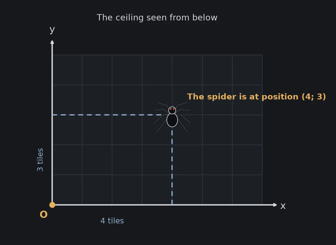
How much of this holds up? The sources I read all call it a legend, and the details vary between tellings: one says he was in bed, another says the ceiling was tiled[7][8]. I could not find the earliest written source of the anecdote, so I cannot say whether it really happened. One note on the creature: the sources I read tell it with a fly. In this article I tell it with a spider because it is easier to picture, and keep every other detail the same.
Real or not, the anecdote gives a compact picture of the core idea: the position of a point can be stated with two distances measured from two reference lines. But the documented history of how he arrived at that idea is different, and more interesting.
The documented story: the Pappus problem and an “entirely new science”
Descartes’s earliest recorded mathematical thoughts appear in letters exchanged with Isaac Beeckman, whom he met in 1618. In a 1619 letter, he imagined an “entirely new science” that could answer questions about any kind of quantity, continuous or discrete[9].
The concrete turning point came in 1631, when Jacob Golius drew Descartes’s attention to the Pappus problem. That problem became the focus of his exposition of the new method[9]. It is a locus problem with three or four fixed lines in a plane: find every point whose distances to those lines satisfy a condition of proportion[4]. Imagine you want every spot where a coffee shop could stand so that its distances to three main roads always keep a fixed ratio. With a ruler and compass, it is hard to tell what shape those spots make.
Descartes solved it like this[9]. He assumed a point C lies on the locus, then drew segments from C to the four given lines. He took the segment AB, measured from a fixed point A, as the first unknown, called x. The segment BC was the second unknown, called y. The point C traces the locus as BC slides along AB while keeping a fixed angle. Every other distance could be expressed through x and y, and the condition of proportion became one equation between x and y. That equation tells you what curve the locus is.
That was the real leap. Descartes did not draw two perpendicular axes. He chose the axes to suit each problem, and according to Encyclopedia.com, the “Cartesian coordinate system” does not appear anywhere in La Géométrie, so the name is a misnomer[9]. What he did was turn a curve into an equation.
Comparing the two stories: the spider anecdote gives us the idea “two distances pin down a point” in a single moment. The documented history gives a longer path: an idea for a new science in 1619, then a concrete problem in 1631 that forced him to find a method.
Who was Descartes?
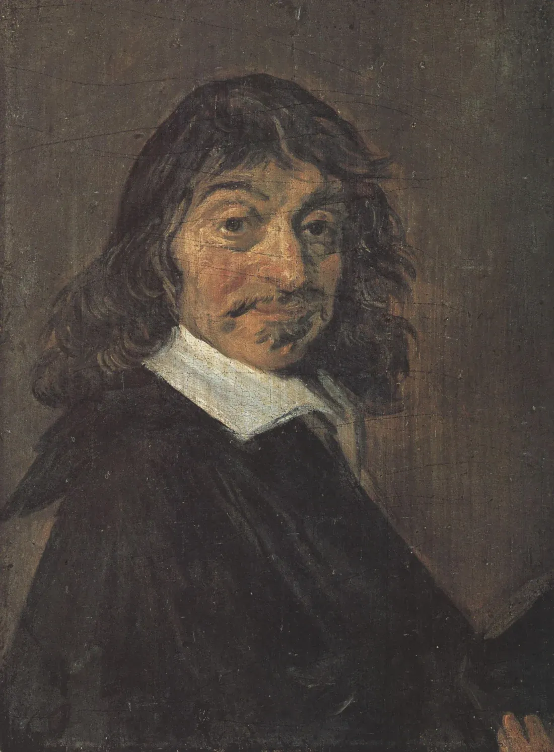
René Descartes was born in 1596 in La Haye en Touraine, France[3]. He published his work while living in the Netherlands[2].
In 1630 he enrolled at Leiden University under the name “Poitevin.” That same year he fell out with Isaac Beeckman, whom he accused of plagiarizing some of his ideas[3]. In 1633, news came from Italy to the Netherlands: Galileo had been condemned by the Inquisition. Descartes then had a manuscript about the universe and physics, called Treatise on the World. According to biographies, after the condemnation he abandoned plans to publish it[3].
In 1637 he published parts of that work as three essays, preceded by an introduction, the Discours de la méthode (Discourse on the Method), printed in Leiden[1][3]. The three essays are La Dioptrique (Optics), Les Météores (Meteorology) and La Géométrie (Geometry)[1]. Descartes wrote in French, not in Latin, which was the language of scholars at the time[4]. La Géométrie is where the idea of this article lives.
His relations with universities were not smooth. In 1643 his philosophy was condemned at the University of Utrecht, and he had to move to The Hague[3]. In 1649 Queen Christina of Sweden invited him to her court. He accepted and arrived in Stockholm in the middle of winter, then passed away there in 1650 of pneumonia, although the source also notes that other causes have been proposed[3].
How did geometry and algebra meet?
Before Descartes, geometry and algebra were almost two separate subjects. Geometry was about drawings and lengths. Algebra was about unknown numbers. La Géométrie was the first work to propose merging the two: it reduced geometry to arithmetic and algebra, and translated shapes into equations[4].
Two things in the book are still used today:
- The way of naming. Descartes used letters from the end of the alphabet (x, y, z) for unknown quantities and letters from the beginning (a, b, c) for known ones. The way you write “solve for x” at school still follows this habit[4].
- Turning a geometry problem into an equation. That is exactly what he did with the Pappus problem in the section above. The overview of La Géométrie says the idea of a Cartesian coordinate system can be traced to this work[4].
It is like giving a name to each segment instead of saying “that longish one over there”: once things have names, you can write the equation. Once you have the equation, you can calculate.
But here is the place to correct a familiar misunderstanding. The modern perpendicular coordinate system does not appear in La Géométrie. According to the overview of the coordinate system, Descartes and Fermat both used a single axis, with variable lengths measured from it[2]. Using a pair of axes was brought in after La Géométrie was translated into Latin in 1649 by Frans van Schooten and his students, who clarified Descartes’s ideas further[2][4]. The 1659–1661 edition is more than twice the length of the original, with explanations and examples added by van Schooten and his students[4]. One person before both Descartes and Fermat, the cleric Nicole Oresme, used similar constructions long before them[2].
So the more accurate statement is: Descartes laid the foundation for turning geometry into algebra. The x-y system as we draw it on the board is the product of many people, formed gradually after him.
Fermat: the man with the same idea who did not publish
Descartes was not alone. Pierre de Fermat found the idea of coordinates independently, and even worked in three dimensions, but did not publish[2]. According to Descartes’s biography, La Géométrie exploited discoveries he made together with Fermat[3]. The two also tested each other: in 1638, Descartes challenged Fermat to find the tangent of the folium of Descartes, and Fermat solved it easily while Descartes could not[5].
Seen this way, the question “who came up with the x-y axes” really has no single answer. The idea appeared in several places almost at once, and the person who published first, with a book strong enough to spread widely, is the one who got the name. The article Who is the father of the computer? tells a story of the same kind: one name stands out, but many people contributed.
What changed in how we see geometry?
Before La Géométrie, a shape was something you constructed with a ruler and compass, then proved its properties through geometric arguments. Afterward, a shape was also something you wrote as an equation, and its properties could be read from the equation.
Three concrete changes:
- A curve becomes an equation. Instead of describing a circle as “every point at distance 5 from O,” we write . The geometric condition and the algebraic condition are one. It is like turning a paper map into a table of numbers: all the information is still there, but now a computer can work with it.
- A geometry problem becomes an equation-solving problem. To find where two shapes meet, we solve the system of their equations instead of drawing them as precisely as we can. See the example in the section below.
- Curves are classified by their equations. Descartes was interested in classifying curves by the degree of their equations[5]. A circle and a line have low-degree equations, and the folium of Descartes has degree three. Geometry thereby gained a way of sorting that a ruler and compass cannot give.
For you, the nearest consequence is that every graph you drew at school is the picture of an equation. The farther consequence is location maps, 3D graphics and artificial intelligence, as the application section below shows.
What does the equation of a line tell you?
Before solving the intersection problem, let us revisit the simplest equation. is a rule: pick a value of x, add 1, and you get the value of y. With x = 0 we get y = 1, with x = 1 we get y = 2, with x = 2 we get y = 3. The three points (0; 1), (1; 2), (2; 3) lie on the same line, and the point A(2; 3) from the start of this article is one of them.
Rules like this are familiar outside school. Suppose a taxi company (illustrative figures) charges 12,000 dong to start plus 10,000 dong per kilometer: the fare is , where x is the number of kilometers. Every trip is a point, and all trips lie on one line. The coefficient 10,000 is the slope: for every extra kilometer, the line rises by 10,000 dong.
What Descartes saw is this: if every line is a rule like that, and every curve is also a rule, only a more complicated one, then we can do math with the rules instead of drawing pictures.
Algebra solving geometry: a school problem
Let us try an example to see how it works. A circle centered at O with radius 5 has the equation . The line passes through the point (0; 1) and through the point A(2; 3) from the start of this article. Where do the two shapes meet?
No compass or ruler is needed. Substitute into the circle’s equation: , which is , or . This equation has two solutions, and . So the two intersections are (3; 4) and (−4; −3). The code at the end of the article checks that both points satisfy .
Did you notice (3; 4) and the radius 5? That is the familiar Pythagorean triple 3, 4, 5. In pure geometry, you would have to construct a figure to see it. In algebra, it appears from solving a quadratic equation.
If the axes did not exist, what else could not?
An idea from 1637 sounds small, but the four things below all run on it. They look very far apart: rockets, the map on your phone, a 3D character, a chatbot. What they share is that each one turns what needs to be computed into a list of numbers on a coordinate system.
Calculus, aviation and spaceflight
According to the overview, analytic geometry (another name for coordinate geometry) is the foundation of most modern fields of geometry, including algebraic, differential, discrete and computational geometry. It is also used in physics, engineering, aviation, rocketry, space science and spaceflight[11]. La Géométrie in particular is credited with providing a foundation for calculus in Europe[11]. My reading of why: an orbit is a curve, and only when the curve is an equation can you compute the velocity and heading at each point along it.
GPS: your phone solves a system of equations
GPS satellites orbit at an altitude of about 20,200 km. The nominal design has 24 satellites in six orbital planes with four satellites each, and about 31 satellites are operational today[10]. Every time you open a map, the receiver measures the time a signal takes to travel from each satellite, converts it into a distance, and from those distances solves for three position coordinates plus its own clock offset. With four unknowns, the receiver needs to see at least four satellites[10]. The solution is computed in Earth-centered Cartesian coordinates, and only then converted to latitude, longitude and height[10].
A simple picture: you stand in a yard and know you are 10 meters from the first flagpole, 20 meters from the second and 30 meters from the third. Each distance is a circle around a pole, and where they meet shows exactly where you stand. This is an example I made up for illustration, in the same spirit as the circle-meets-line problem above, but GPS works in three dimensions.
On accuracy: after the deliberate degradation was turned off on May 1, 2000, civilian GPS reached about 5 meters. Receivers using the L5 band reach about 30 cm, and phones can reach 4.9 meters or better when assisted by Wi-Fi[10]. The article on GPS and relativity explains why the satellite clocks must be corrected.
3D graphics: a character is a very long table of numbers
In computer graphics, a 3D object is usually described by a polygon mesh: a collection of vertices, edges and faces that define the surface of the object. Each vertex is a position given by three coordinates (x, y, z)[13]. The list of faces is usually sent to the GPU as indices into the vertex list, and that is the data form modern graphics hardware typically takes as input[13]. So what you see on screen as a face or a car is, to the GPU, rows of (x, y, z) numbers. The article on CPUs and GPUs explains why a GPU suits this kind of work.
Artificial intelligence: meaning becomes position
The idea “a thing is a point” goes further than geometry. A word embedding represents each word with a vector of many real numbers, and words that sit close together in that space are expected to have similar meanings[6]. Word2vec, published by a team led by Tomáš Mikolov at Google in 2013, produces vectors that typically have several hundred dimensions, in a range of 100 to 1,000[12]. Words that often appear in the same contexts end up close together, and relationships in meaning can be reproduced with vector addition and subtraction. An example from the overview itself: take the vector for “Brother,” subtract “Man,” add “Woman,” and the closest vector is “Sister”[12].
Instead of two coordinates like the point A(2; 3), a word has hundreds, but the principle is the same: position in a space tells you the relationships. The idea of learning to represent words as vectors with neural networks is older: in 2000, Bengio and colleagues published work along those lines[6]. The articles on cosine similarity and vector databases explain how closeness is measured and how these points are stored.
A question from 7th grade, “why do we need the x and y axes,” turns out to be a question that all four of these things answer in their own way.
Three common misunderstandings about Descartes
Did he come up with the axes while watching a spider on the ceiling? That is a legend, and the sources I read do not confirm it[7][8]. What is documented is that he reached the idea through the Pappus problem in 1631[9].
Did Descartes invent the x-y axes? Nearly, but not exactly. He laid the foundation for turning geometry into algebra in La Géométrie, but the modern system of two perpendicular axes is not in that book. It formed gradually afterward, with contributions from Fermat, van Schooten and others[2][4].
Could he solve every problem he set himself? No. In 1638, Descartes studied a curve now called the folium of Descartes and challenged Fermat to find the tangent at an arbitrary point. According to the overview, Fermat solved it easily, and Descartes could not[5]. Today, implicit differentiation makes this straightforward.
The notation, compactly
This part is for readers who want the formulas. Skipping it does not lose the main idea.
A point in the plane is a pair of numbers . The circle centered at O with radius :
The folium of Descartes has the equation[5]:
Setting gives the parametric form , . The loop of the leaf corresponds to . The curve has the asymptote and is symmetric about the line [5]. The area of the loop equals [5].
Implicit differentiation gives the slope of the tangent at a point on the curve:
Solve the intersection and draw the folium yourself
The Python script below does three things. It solves the intersection of the circle and the line , draws the folium of Descartes with its asymptote, then computes the area of the loop by numerical integration to compare with the formula , and computes the slope of the tangent at the point (1.5; 1.5). It draws Figure 3. There is no randomness, so no seed is needed. You need numpy and matplotlib.
import matplotlib.pyplot as pltimport numpy as np
plt.rcParams.update({"figure.facecolor": "#16181c", "axes.facecolor": "#16181c", "text.color": "#d4d7dc",                     "axes.edgecolor": "#2a2e35", "axes.labelcolor": "#a4a9b2",                     "xtick.color": "#878d97", "ytick.color": "#878d97", "font.size": 12})
# Part 1: algebra solves a geometry problem. Where does the line y = x + 1 cut the circle x² + y² = 25?# Substitute y = x + 1 into the circle: x² + (x + 1)² = 25, which is 2x² + 2x - 24 = 0.x_cut = np.sort(np.roots([2, 2, -24]))y_cut = x_cut + 1for x, y in zip(x_cut, y_cut):    print(f"intersection: ({x:.0f}; {y:.0f}), check x² + y² = {x ** 2 + y ** 2:.0f}")
# Part 2: the folium of Descartes x³ + y³ = 3axy, with a = 1.a = 1.0
# Area of the loop: use polar coordinates r(θ) = 3a·sinθ·cosθ / (sin³θ + cos³θ), θ from 0 to π/2, S = ½ ∫ r² dθ.theta = np.linspace(1e-9, np.pi / 2 - 1e-9, 200_001)r = 3 * a * np.sin(theta) * np.cos(theta) / (np.sin(theta) ** 3 + np.cos(theta) ** 3)loop_area = 0.5 * np.trapezoid(r ** 2, theta)print(f"loop area (a = 1): {loop_area:.4f}, formula 3a²/2 = {1.5 * a ** 2:.4f}")
# Tangent at (1.5; 1.5): implicit differentiation gives dy/dx = (a·y - x²) / (y² - a·x), the task Descartes once set Fermat.x0 = y0 = 1.5 * aslope = (a * y0 - x0 ** 2) / (y0 ** 2 - a * x0)print(f"slope of the tangent at ({x0}; {y0}): {slope:.2f}")
# Drawfig, (ax1, ax2) = plt.subplots(1, 2, figsize=(14, 6.4), gridspec_kw={"wspace": 0.18})
# Left: the x and y axes, the circle, the line, the two intersections and the point A(2; 3).phi = np.linspace(0, 2 * np.pi, 400)ax1.plot(5 * np.cos(phi), 5 * np.sin(phi), color="#8fa9c9", lw=2.4)xs = np.array([-6.5, 6.5])ax1.plot(xs, xs + 1, color="#e8b05a", lw=2.4)ax1.scatter(x_cut, y_cut, color="#f4e9d2", s=70, zorder=4)for x, y, dx, dy in zip(x_cut, y_cut, (-1.6, 0.3), (-0.9, 0.5)):    ax1.annotate(f"({x:.0f}; {y:.0f})", (x, y), xytext=(x + dx, y + dy), color="#f4e9d2", fontsize=12)ax1.scatter([2], [3], color="#c9884a", s=70, zorder=4)ax1.annotate("A(2; 3)", (2, 3), xytext=(2.2, 2.0), color="#c9884a", fontsize=12)ax1.axhline(0, color="#d4d7dc", lw=1.4)ax1.axvline(0, color="#d4d7dc", lw=1.4)ax1.text(6.6, 0.2, "x", color="#d4d7dc", fontsize=13)ax1.text(0.2, 6.6, "y", color="#d4d7dc", fontsize=13)ax1.text(-0.65, -0.75, "O", color="#d4d7dc", fontsize=13)ax1.set_xlim(-7, 7.3)ax1.set_ylim(-7, 7.3)ax1.set_aspect("equal")ax1.grid(color="#2a2e35", lw=0.8)ax1.set_title("The circle x² + y² = 25 meets the line y = x + 1", color="#d4d7dc", fontsize=12.5)
# Right: the folium of Descartes, its loop, the asymptote and the tangent.g = np.linspace(-2.6, 3.2, 1600)X, Y = np.meshgrid(g, g)ax2.contour(X, Y, X ** 3 + Y ** 3 - 3 * a * X * Y, levels=[0], colors=["#e8b05a"], linewidths=2.6)ax2.fill(r * np.cos(theta), r * np.sin(theta), color="#c9884a", alpha=0.55)xt = np.array([-2.2, 3.0])ax2.plot(xt, -xt - a, color="#8fa9c9", lw=1.8, ls=(0, (4, 3)))ax2.plot(xt, y0 + slope * (xt - x0), color="#f4e9d2", lw=1.6)ax2.scatter([x0], [y0], color="#f4e9d2", s=60, zorder=4)ax2.annotate("tangent at (1.5; 1.5)", (x0, y0), xytext=(1.0, 2.55), color="#f4e9d2", fontsize=12)ax2.annotate("asymptote x + y + 1 = 0", (-2.5, -1.7), color="#8fa9c9", fontsize=12)ax2.text(1.45, 0.45, f"loop, area\n{loop_area:.2f}", color="#f4e9d2", fontsize=12)ax2.axhline(0, color="#d4d7dc", lw=1.0)ax2.axvline(0, color="#d4d7dc", lw=1.0)ax2.set_xlim(-2.6, 3.2)ax2.set_ylim(-2.6, 3.2)ax2.set_aspect("equal")ax2.grid(color="#2a2e35", lw=0.8)ax2.set_title("Folium of Descartes x³ + y³ = 3xy (a = 1)", color="#d4d7dc", fontsize=12.5)for a_ in (ax1, ax2):    for sp in ("top", "right"):        a_.spines[sp].set_visible(False)fig.savefig("descartes-oxy-en.png", dpi=150, bbox_inches="tight")
Output:
intersection: (-4; -3), check x² + y² = 25intersection: (3; 4), check x² + y² = 25loop area (a = 1): 1.5000, formula 3a²/2 = 1.5000slope of the tangent at (1.5; 1.5): -1.00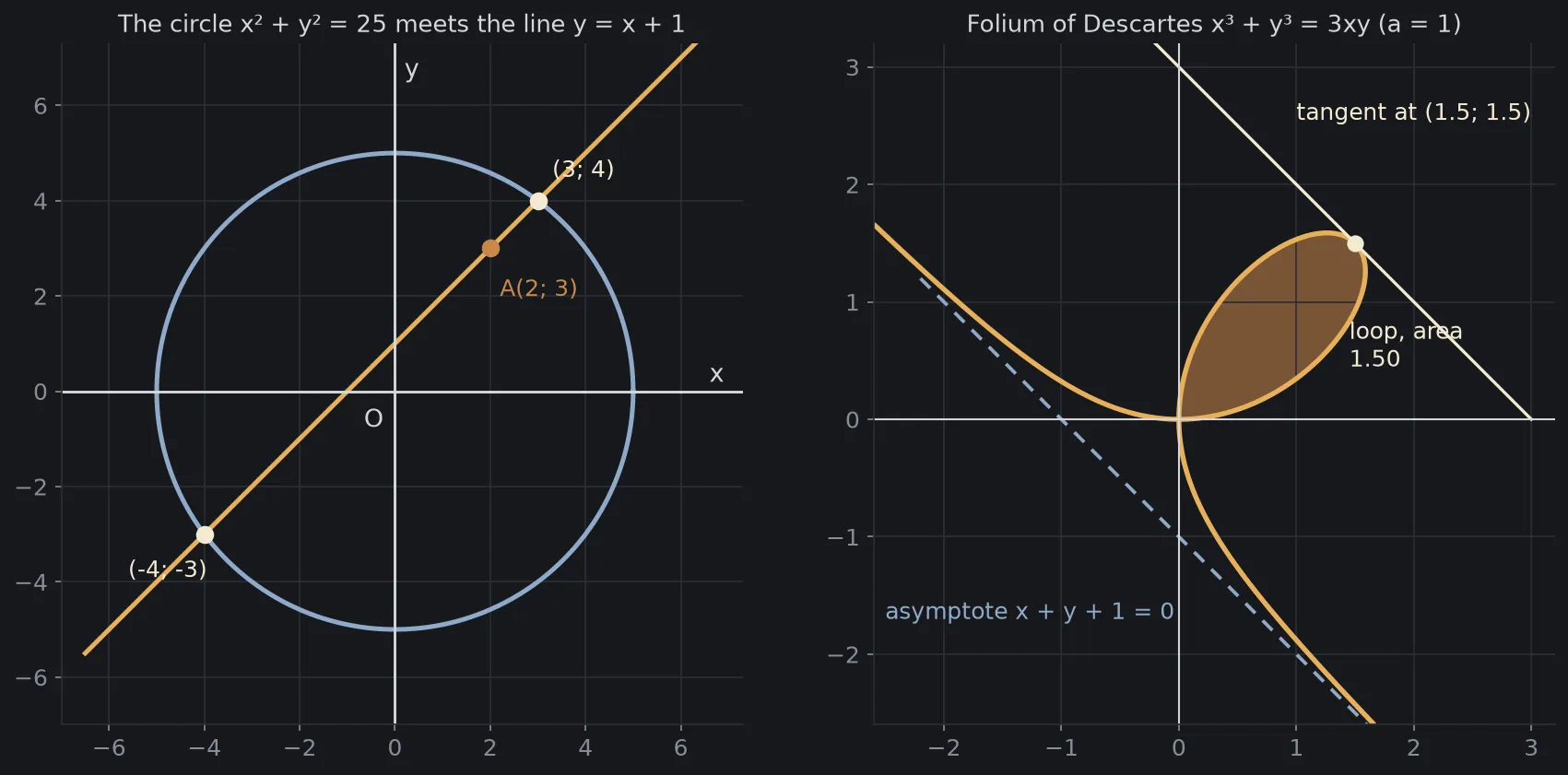
The first two lines confirm the algebraic solution: both (3; 4) and (−4; −3) satisfy the circle’s equation. The third line shows that the numerical integral matches the formula: the loop area is 1.5 when . The last line gives a slope of −1 at (1.5; 1.5), exactly what implicit differentiation in the notation section gives: . The shape of the leaf is also worth a closer look: the curve has a loop in the first quadrant, a double point at the origin O, is symmetric about the line , and meets that line at the origin and at the point [5]. The name “folium” is Latin for “leaf”[5]. You can change a to 2 or 0.5 to watch the loop grow or shrink, or change the line to to see where it meets the circle.
Back to the point A(2; 3)
The point A(2; 3) at the start of this article is no longer just two numbers. It is the result of an idea tested on an ancient problem in 1631: call the unknown segments x and y, then let the equation tell you what curve the locus is. From then on, geometry had one more way of working, beside the ruler and compass.
Why do we need the x and y axes? Because with them, every shape has an equation, and every equation can be solved by calculation. Descartes laid the foundation for that idea in 1637, and it changed how we see geometry: from something to draw into something to calculate.
Free geometry illustrations for students and teachers: EyeViz.
Tài liệu tham khảo
- [1]Discourse on the Method. Wikipedia.
- [2]Cartesian coordinate system. Wikipedia.
- [3]René Descartes. Wikipedia.
- [4]La Géométrie. Wikipedia.
- [5]Folium of Descartes. Wikipedia.
- [6]Word embedding. Wikipedia.
- [7]Maths in a minute: Cartesian coordinates. Plus Maths, University of Cambridge.
- [8]Cartesian coordinates. Encyclopaedia Britannica.
- [9]Descartes, René: mathematics and physics. Encyclopedia.com.
- [10]Global Positioning System. Wikipedia.
- [11]Analytic geometry. Wikipedia.
- [12]Word2vec. Wikipedia.
- [13]Polygon mesh. Wikipedia.