Grade inflation: what share of top degrees is reasonable?
What is grade inflation, what share of top degrees is reasonable, and what does the normal distribution say? From graduation day to credit ratings.
Mục lục
A graduation ceremony where half the graduates get a top degree
One morning in August, a graduation ceremony at a certain university. The host reads each student’s name, and for every two graduates who walk across the stage, one receives an “excellent” degree. Parents clap steadily. But in the row for employers, someone leans over to the person beside them and asks: so among these graduates, who is really at the top?
That is the question of this article: what share of top degrees is reasonable, and when the share rises, how much can the “excellent” label still tell people apart. The short answer: there is no single nice number for every place. The reasonable share depends on what the label is used for. If the label is used to pick out standouts, it has to go to a small group, around 5 to 10%. If the label only certifies that a standard has been met, it can go to many people, but then you need another signal to tell them apart.
This article uses the normal distribution to work out the cutoff for each top group, runs a simulation to show how a label loses its selectivity when it goes to more people, and then compares it with a phenomenon of the same nature in investing: credit rating inflation.
What is a top degree for?
A degree actually does two different jobs, and we often mix them up.
The first job is certification: this person has met a standard. Like a driver’s license, anyone who passes the test gets one, with no cap on how many people. The second job is ranking: where this person stands compared with others. Like placing in a race, only a few people at the top get medals.
Under Vietnam’s current regulation on undergraduate education, an excellent degree corresponds to a cumulative grade point average of 3.60 to 4.00 on a 4-point scale, a good degree to 3.20 up to below 3.60, and a fair degree to 2.50 up to below 3.20[6]. This is an absolute standard. In principle, if every student meets the standard, every student can get an excellent degree. But employers read the same degree the second way: “this person is in the top group.” The two readings only match when the excellent label goes to a small group.
What does the normal distribution say about the top group?
Picture the exam scores of a large class. Most students sit around the average, and the further from the average, the fewer the students, evenly on both sides. That shape is called the normal distribution (the bell curve). About 68% of values lie within one standard deviation of the mean, about 95% within two, and about 99.7% within three[4]. The standard deviation measures spread: think of it as the width of a crowd around the center line of a field.
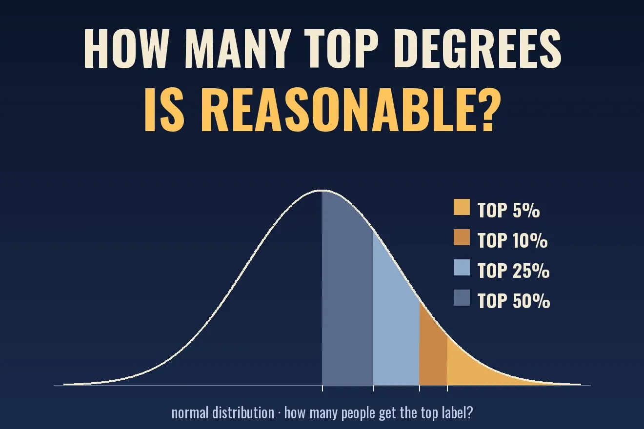
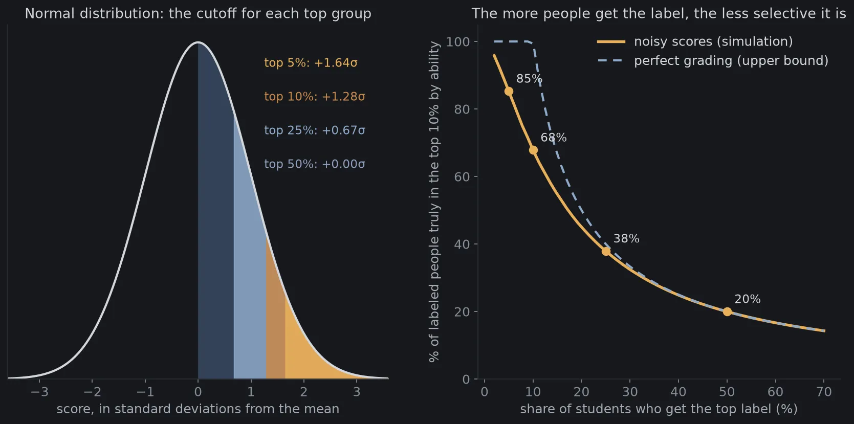
When data really is normally distributed, we can compute the cutoff for each top group. Results from the code at the end of the article:
| Top group | Score cutoff |
|---|---|
| Top 5% | mean + 1.64 standard deviations |
| Top 10% | mean + 1.28 standard deviations |
| Top 25% | mean + 0.67 standard deviations |
| Top 50% | exactly at the mean |
The last row is the one to notice: a label that goes to 50% of students has its cutoff right in the middle of the crowd. The person just above the center line and the person just below it are almost no different, yet one has the top label and the other does not.
A limit needs saying right away: the normal distribution appears when a quantity is the sum of many small independent factors, and it is often misused for data that is strongly skewed or capped[4]. A cumulative GPA is capped at 4.0, so it cannot be exactly normal. We use the normal distribution as a reference point, not as a law that scores must follow.
The more people get the label, how selective is it?
Suppose an employer wants to find the 10% of students who are strongest in true ability. They use the “excellent” label as a filter. If the label goes to exactly 10% and scores reflect ability perfectly, everyone with the label is in the top 10%. If the label goes to 50%, then even with perfect scores, at most 1 in 5 people with the label is in the top 10%, because 50% is five times 10%.
Reality is worse, because scores never reflect ability perfectly: exams are a matter of luck, graders differ, there are good days and bad days. This noise is also why whoever finished first this time tends to do worse next time, as the article on regression to the mean (article in Vietnamese) explains. I simulated 200,000 students, each with a true ability drawn from a normal distribution. Their score equals ability plus grading noise with a standard deviation of 0.5. Results, among people who have the label:
| Label goes to | Truly in the top 10% by ability (noisy) | Upper bound (perfect grading) |
|---|---|---|
| 5% | 85% | 100% |
| 10% | 68% | 100% |
| 25% | 38% | 40% |
| 50% | 20% | 20% |
When the label goes to 5%, most people with the label are the strongest. When it goes to 50%, only about 1 in 5 people with the label is in the top 10%, however good the grading is. That is what the employer in the back row senses: the label no longer tells them much.
An everyday example: a restaurant where everyone gets 5 stars. Diners can still read 5 stars, but they cannot tell which place is really good. To tell them apart, they have to look for other signals: detailed reviews, how many people book a table.
What do the news reports say about grade inflation?
Grade inflation is the awarding of higher grades for the same quality of work over time, which devalues grades[3]. A distinction matters: a rise in average grades alone does not prove inflation. To prove it, you have to show the work does not deserve the higher grade[3].
In Vietnam, the issue was widely discussed in October 2026. According to the press, at a higher education conference on October 1, 2026, the Minister of Education and Training voiced concern that the rates of good and excellent graduates are rising at many schools while the actual quality is unclear. On October 16, 2026, the Ministry told universities to review student learning outcomes and not to impose quotas on good and excellent ratings[1]. According to a CafeF report, schools were asked to analyze grade distributions by major, cohort and form of training, check them against learning outcomes and employer feedback, and not lower standards to chase achievement figures[2].
Around the same time, an article compiling graduation announcements for 2025 and 2026 reported large gaps among fields. At many economics and finance schools, good and excellent graduates make up roughly three quarters of the class or more. At some engineering schools, the excellent rate is only a few percent. At some medical schools, some graduating classes had no excellent graduates at all[1].
That article offers no independent analysis of the causes of the gap[1]. I do not speculate further either. What can be drawn from the figures themselves is this: the rates differ very widely between fields, from a few percent to more than half the class, so the excellent rate cannot yet be compared directly between places.
Is a lot of top degrees necessarily bad?
No. There are at least three legitimate reasons why a high rate can exist without inflation.
First, criterion-referenced grading differs from norm-referenced grading (grading on a curve). If a school sets a clear standard and students truly meet it, many excellent graduates is the correct result, and there is no need to force a bell-shaped distribution. Second, the quality of incoming students can rise over time. Third, converting from a 10-point scale to a 4-point scale squeezes many different scores into the same band.
So how do you recognize inflation? Not from the rate alone. You have to compare the same level of work across years, or check against an outside measurement: a common exam, cross-marking of exam papers, or outcomes after graduation. Those are exactly the things the Ministry asked schools to do: sample exam papers and check against employer feedback[2].
A foreign example shows that a rate can also be pulled back when a school sets a policy. A university in the United States set out to reduce the share of A grades: it fell from 47.9% in the 2002–03 school year to 39.7% in 2008–09[3]. The example does not say the policy was good or bad. It only shows the rate is something that can be adjusted through grading standards.
It is also worth knowing the cost of grades piling up. One compiled source reports that when grades are pushed up, a student at the 98th percentile and a student at the 82nd percentile can become indistinguishable[3]. This is information compression: the grade bands stay the same, but the real distances between students are hidden.
The same mechanism in investing: rating inflation
A top label going to too many cases also happens in finance. The clearest example is the credit rating: AAA is the highest grade, meaning the lowest risk of default.
From 2000 to 2007, the rating agency Moody’s rated nearly 45,000 mortgage-related securities triple-A, more than half of the securities of this kind it rated. According to authors cited on the page, 70% to 80% of new tranches of structured debt products (CDOs) were rated AAA, even though the underlying bonds were mostly only BBB or A-minus. By April 2010, according to the U.S. Financial Crisis Inquiry Commission, 73% of the mortgage-backed securities that Moody’s rated AAA in 2006 had been downgraded to junk[5]. Some figures here come from journalistic books or secondary citations, so treat them as a sense of scale rather than exact numbers[5].
The cause usually named is a conflict of interest: investment banks paid the rating agencies fees to obtain the rating they wanted, and a study of 6,500 ratings found that ratings were biased toward issuers who brought the agencies more business[5].
The link to our problem is fairly direct. When AAA goes to the majority, an investor cannot use the label to pick out the safest part. They have to look for other signals: analyzing the underlying assets themselves, the spread over government bond yields, or their own asset valuation techniques. This is also like an employer who cannot rely on the excellent label alone.
Three common misunderstandings
Does a high excellent rate mean there is definitely inflation? Not necessarily. As said, grading standards, student intake and the way scores are converted all matter. To conclude, you need an outside measurement or a comparison of the same level of work over time[3].
Do scores have to follow a normal distribution to be “good”? No. The normal distribution is a useful reference for computing cutoffs, but scores are capped at the top, and criterion-referenced grading does not need a bell shape[4]. What is needed is for the top label to still say something.
Is it enough to fix the share of excellent degrees by rule? Not quite. The management documents reported in the press themselves say not to impose quotas[1]. The reason is easy to see: if the share is fixed, the label can be used for internal comparison, but it can no longer say whether a whole cohort got better or worse. When a measure becomes a target, people optimize the measure instead of what it measures.
The notation, compactly
This part is for readers who want the formulas. Skipping it does not lose the main idea.
If scores follow a normal distribution with mean and standard deviation , the cutoff of the top share is
where is the inverse of the standard normal distribution function. For we have .
If scores reflect the ranking of ability perfectly and the label goes to the top share, the share of labeled people who belong to the top share by ability is
For example, and give , matching the last row of the table. When scores are noisy, the precision lies below this bound.
Simulate it yourself
The Python script below computes the cutoffs of the top groups with the normal distribution, simulates 200,000 assumed students with true ability and grading noise, then measures the selectivity of the top label. It draws Figure 1. The figures are entirely assumed and the model is very simple: it assumes normally distributed ability and additive noise, while real scores are capped and can be skewed. The noise level of 0.5 is my own choice. The seed is fixed (2026), so rerunning gives identical results. You need numpy and matplotlib.
from statistics import NormalDist
import matplotlib.pyplot as pltimport numpy as np
plt.rcParams.update({"figure.facecolor": "#16181c", "axes.facecolor": "#16181c", "text.color": "#d4d7dc",                     "axes.edgecolor": "#2a2e35", "axes.labelcolor": "#a4a9b2",                     "xtick.color": "#878d97", "ytick.color": "#878d97", "font.size": 12})
NORMAL = NormalDist()                     # standard normal distribution: mean 0, standard deviation 1SHARES = [0.05, 0.10, 0.25, 0.50]         # the top label goes to the top 5%, 10%, 25%, 50% of students
# Part 1: the score cutoff (in standard deviations above the mean) for each top groupfor p in SHARES:    print(f"top {p:.0%}: cutoff = mean + {NORMAL.inv_cdf(1 - p):.2f} standard deviations")
# Part 2: simulation. True ability ~ standard normal; score = ability + grading noise (standard deviation 0.5).rng = np.random.default_rng(2026)N = 200_000ability = rng.standard_normal(N)score = ability + 0.5 * rng.standard_normal(N)true_top10 = ability >= np.quantile(ability, 0.90)     # the 10% most able by true ability

def precision(share, s=score):    """Among people who get the label (top group by score), what percent are truly in the top 10% by ability."""    labeled = s >= np.quantile(s, 1 - share)    return true_top10[labeled].mean()

print("label given to   precision (noisy)   precision (perfect grading)")for p in SHARES:    ideal = min(1.0, 0.10 / p)    print(f"{p:>12.0%}   {precision(p):>16.0%}   {ideal:>24.0%}")
# Drawfig = plt.figure(figsize=(14, 6))o = fig.add_gridspec(1, 2, width_ratios=[1.05, 1], wspace=0.24)
ax = fig.add_subplot(o[0])x = np.linspace(-3.6, 3.6, 600)y = np.exp(-x ** 2 / 2) / np.sqrt(2 * np.pi)ax.plot(x, y, color="#d4d7dc", lw=2)colors = {0.05: "#e8b05a", 0.10: "#c9884a", 0.25: "#8fa9c9", 0.50: "#3a4a63"}for p in SHARES[::-1]:    z = NORMAL.inv_cdf(1 - p)    ax.fill_between(x, 0, y, where=x >= z, color=colors[p], alpha=0.85)for p, dy in zip(SHARES, (0.37, 0.33, 0.29, 0.25)):    z = NORMAL.inv_cdf(1 - p)    ax.text(1.25, dy, f"top {p:.0%}: +{z:.2f}σ", color=colors[p] if p < 0.5 else "#8fa0bd", fontsize=11)ax.set_xlim(-3.6, 3.6)ax.set_ylim(0, 0.42)ax.set_yticks([])ax.set_xlabel("score, in standard deviations from the mean")ax.set_title("Normal distribution: the cutoff for each top group", color="#d4d7dc", fontsize=13)
ax = fig.add_subplot(o[1])shares = np.linspace(0.02, 0.70, 60)ax.plot(shares * 100, [precision(p) * 100 for p in shares], color="#e8b05a", lw=2.6, label="noisy scores (simulation)")ax.plot(shares * 100, [min(1, 0.10 / p) * 100 for p in shares], color="#8fa9c9", lw=2, ls=(0, (4, 3)),        label="perfect grading (upper bound)")for p in SHARES:    v = precision(p) * 100    ax.scatter([p * 100], [v], color="#e8b05a", s=55, zorder=3)    ax.annotate(f"{v:.0f}%", (p * 100, v), xytext=(7, 8), textcoords="offset points", color="#d4d7dc", fontsize=11)ax.set_xlabel("share of students who get the top label (%)")ax.set_ylabel("% of labeled people truly in the top 10% by ability")ax.set_ylim(0, 105)ax.legend(frameon=False, loc="upper right")ax.set_title("The more people get the label, the less selective it is", color="#d4d7dc", fontsize=13)for a_ in fig.axes:    for sp in ("top", "right"):        a_.spines[sp].set_visible(False)fig.savefig("lam-phat-diem-en.png", dpi=150, bbox_inches="tight")
Output:
top 5%: cutoff = mean + 1.64 standard deviationstop 10%: cutoff = mean + 1.28 standard deviationstop 25%: cutoff = mean + 0.67 standard deviationstop 50%: cutoff = mean + 0.00 standard deviationslabel given to precision (noisy) precision (perfect grading) 5% 85% 100% 10% 68% 100% 25% 38% 40% 50% 20% 20%You can change the factor 0.5 in the line that computes score to try other noise levels. The more noise, the further the gold line moves from the upper bound. You can also change 0.90 in true_top10 to 0.95 to ask about the top 5% instead of the top 10%.
Back to the graduation ceremony
The person who leaned over in the employers’ row did not ask the wrong question. He was asking about something that an “excellent” label, when it goes to half the graduates, struggles to answer. The label itself is not at fault: it still certifies that those students met the school’s standard.
To make the label say more, there are two directions, and both can be used together. One is to tie the standard of the label to a smaller group. The other is to add a separate signal for the larger group, such as rank within the cohort or a common assessment, so readers know who stands where. This article does not say which direction is right. It only shows that a label given to half the crowd needs something else to go with it.
Free geometry illustrations for students and teachers: EyeViz.
Tài liệu tham khảo
- [1]Doãn Nhàn. Chênh lệch tỷ lệ tốt nghiệp giỏi, xuất sắc giữa một số trường kinh tế - kỹ thuật - y dược (Gap in the rates of good and excellent graduates among some economics, engineering and medical schools; in Vietnamese). Tạp chí điện tử Giáo dục Việt Nam, published October 19, 2026, 2026.
- [2]Siết tình trạng 'lạm phát' điểm số trong trường đại học (Tightening up on grade 'inflation' at universities; in Vietnamese). CafeF, published October 19, 2026, 2026.
- [3]Grade inflation. Wikipedia.
- [4]Normal distribution. Wikipedia.
- [5]Credit rating agencies and the subprime crisis. Wikipedia.
- [6]Circular 08/2021/TT-BGDDT promulgating the Regulation on Undergraduate Education. Ministry of Education and Training of Vietnam, 2021.