Asset valuation techniques: one coffee shop, three prices
Asset valuation techniques include comparables, discounted cash flow and net asset value. See how one coffee shop gets three different prices, and why.
Mục lục
Three people look at a coffee shop
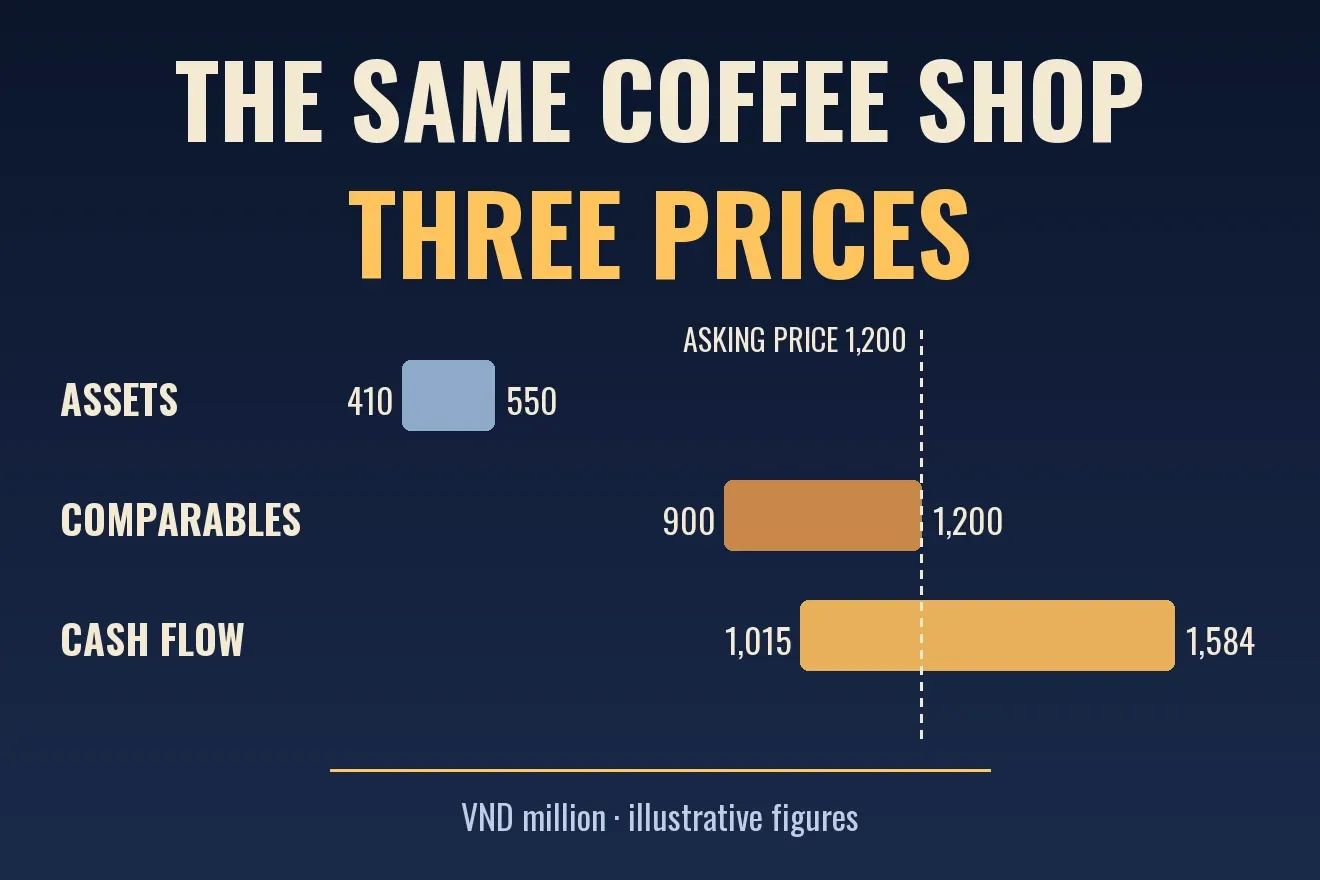
On Saturday morning, a small coffee shop on a street corner puts up a “for sale” sign. The asking price is 1.2 billion Vietnamese dong, including all the equipment and a lease with 8 years left. Three people come to look, and each works out a different number.
The first asks around the neighborhood: what have similar shops sold for recently? The second does not care about other shops. He only asks how much cash this one puts in the owner’s pocket each year. The third goes around counting every coffee grinder, every table and the deposit paid on the premises.
The three are using three valuation techniques. The first compares, the second discounts cash flow, the third adds up assets. The short answer to this article’s question: valuation does not give a single number. It gives a range, and each technique looks at something different: the price of similar things, the money that will flow in later, or what you hold in your hands today.
This article goes through each technique using that same coffee shop, then shows why the three people can all calculate correctly and still land on different results.
What is valuation, and how is it different from market price?
Valuation is an estimate of what an asset is worth. Market price is what people are actually paying for it right now. The two numbers do not have to match. The shop is listed at 1.2 billion dong, but you may think it is worth 900 million or 1.5 billion, and that gap is where the decision to buy or not to buy comes from.
John Burr Williams, who returns in the middle of this article, stressed that real worth and market price are two separate things that an investor should not confuse[3]. Benjamin Graham wrapped the same idea into the image of “Mr. Market”: every day he drops by and offers to buy or sell shares at a different price. You can accept his price or ignore it, and you should pay more attention to how the underlying business is doing[4].
One thing to say early: the overview page on valuation describes it as a subjective exercise, and says all models have limits, because their inputs depend on judgment and assumptions[1]. So the goal is not to find the right number. It is to understand which assumptions each number comes from.
Technique 1: Compare with similar shops
The easiest technique to grasp is to ask what things like it are selling for. You do this whenever you compare house prices in the same neighborhood, or the price of motorbikes from the same year. In finance it is called comparables (also the market approach). Value is inferred from the prices of similar companies, through ratios built on earnings, book value, cash flow or sales[1].
Common ratios:
- P/E (price to earnings): the share price divided by earnings per share. It tells you how many dong you pay for each dong of yearly profit. If the shop earns 300 million a year and sells for 900 million, its P/E is 3.
- P/B (price to book): the price divided by the net asset value recorded in the accounts.
- EV/EBITDA: the value of the whole company, debt included, divided by earnings before interest, taxes and depreciation.
- Some industries have their own ratios. For banks, people look at the net interest margin and loan-loss provisions. For insurers, they look at the value of contracts already on the books[1].
Back to the coffee shop. Suppose similar shops in the area usually sell for about 3 to 4 times annual profit. Our shop earns 300 million a year, so this technique gives about 900 million to 1.2 billion.
It is quick and based on real prices. But it has two weak points. First, it works only if the things being compared are truly alike. The overview page notes that comparables are less accurate for young companies, because each one is different[1]. Second, it inherits the market’s mistakes: if the whole neighborhood is overpaying, you will also compute a high price. And if you only look at shops that are still open, you miss the ones that have closed, a form of survivorship bias (article in Vietnamese).
Technique 2: What is tomorrow’s money worth today?
The second buyer ignores other shops. He only asks: if I buy this shop, what is the money that will come to me over the next 8 years worth today?
The question sounds odd, but you answer it every day. Someone promises to pay you 100 million dong in a year. You could already earn 10% a year by saving, so next year’s 100 million is only worth about 90.9 million today: if you had 90.9 million now and earned 10%, next year you would have exactly 100 million. Converting future money into today’s value is called discounting, and the 10% is called the discount rate.
The discount rate is not just a bank’s interest rate. It reflects the return you demand for taking on risk. A coffee shop is riskier than a savings account, so a buyer might demand 20% a year. The further away and the shakier a payment is, the more it gets discounted.
How it works for the coffee shop, step by step:
- Estimate the money the owner receives each year after all costs: 300 million next year, growing 3% a year.
- Convert each payment to today’s value with a 20% discount rate.
- Add up the 8 payments, plus about 100 million from reselling the equipment at the end of the lease, also discounted.
The result is about 1.27 billion dong. This is discounted cash flow (DCF), also called the income approach: value is the present value of expected cash flows, discounted at a rate that reflects risk and opportunity cost[1].
The man who laid the foundation: John Burr Williams
The idea of discounting future money is very old, as old as lending at interest. The overview page says it was used in the British coal industry from 1801, and that it became popular as a tool for valuing shares after the 1929 crash. Irving Fisher in 1930 and John Burr Williams in 1938 were the two who set it out in modern economic terms[2].
Williams studied mathematics and chemistry at Harvard and worked as a securities analyst. In 1932 he began a PhD in economics, hoping to understand what caused the 1929 Wall Street crash and the Great Depression[3]. His thesis, shaped with help from Joseph Schumpeter, was about the intrinsic value of common stock. It became the book The Theory of Investment Value, printed in 1938 by Harvard University Press[3][5].
Printing the book was not smooth either. Publishers initially refused because of the heavy use of algebraic symbols, and Williams agreed to pay part of the printing cost himself[3]. His main idea: the intrinsic value of a stock is the present value of the dividends it will pay in the future, plus its eventual selling price[3]. He is credited with putting discounted cash flow valuation on solid ground and laying the basis for the dividend discount model. He did not invent the concept of present value itself[3].
How sensitive is the number?
This technique sounds precise, but every input is an assumption. The table in the code section below shows it: for the coffee shop, if the discount rate runs from 15% to 25% and growth from 0% to 5%, the value moves from about 1.0 billion to 1.6 billion. Same shop, same cash flow, and a gap of more than 50%.
For a company assumed to live forever, it is even more sensitive. When cash flow continues indefinitely and grows steadily each year, the value is next year’s cash flow divided by (the discount rate minus the growth rate), and the formula only works when growth is smaller than the discount rate. The overview page says terminal value is highly sensitive to assumptions about growth and the discount rate, and small changes in inputs can produce large changes in the value of a company[2]. In my example, with a 20% discount rate and 3% growth, the value is 1,765 million. Nudge the discount rate up to 21% and the value falls 5.6%. With a 10% discount rate and 5% growth, the value is 6,000 million, and nudging the rate to 11% cuts it by 16.7%. The narrower the gap between the two rates, the smaller the denominator and the more sensitive the value.
Technique 3: Add up the assets, subtract the debts
The third buyer does not look at the future. He asks: if I sold everything in the shop today, how much would I get? This is asset-based valuation (also net asset value): assets minus debts. What remains after an orderly liquidation is treated as a floor for the value[1].
The coffee shop has equipment worth 250 million, furniture worth 100 million and a premises deposit of 200 million. On paper that totals 550 million. But used machines and furniture usually resell below what they cost. If we assume they resell at 60%, the liquidation value is 410 million. This technique gives a range of 410 to 550 million.
It is useful when a company may have to be sold off, or when assets are the main source of value (like a company holding real estate). It is weak for a business whose value sits in things that are hard to count: brand, regular customers, location. The overview page also says intangible assets rarely have observable sale prices, so valuing them is often slow and costly[1]. This coffee shop earns 300 million a year from exactly those intangible sources, and adding up assets does not see them.
Two more techniques, briefly
The dividend discount model is the version of discounted cash flow for shares: instead of the company’s cash flow, you discount the dividends you receive, plus the eventual sale price. That is the idea in Williams’s 1938 book[3].
Contingent claim valuation is for assets with option-like features, such as warrants, employee stock options or callable bonds. People use models such as Black–Scholes–Merton, lattice models or Monte Carlo simulation[1]. This article does not go deeper into that group.
Which technique for which kind of asset?
There is no best technique, only the technique that suits each kind of asset. The table below is a suggestion for where to start, not a hard rule.
| Kind of asset | Usually start from | Note |
|---|---|---|
| Business with steady profits | Discounted cash flow, plus comparables | Check sensitivity to the discount rate and growth |
| Banks and financial firms | P/E, P/B | A bank’s debt is more like raw material than capital, so enterprise value (EV) is less useful[1] |
| Young companies | Discounted cash flow with several scenarios | Comparables are less accurate because each company is different[1] |
| Companies about to be liquidated, or asset-heavy ones | Net asset value | The floor of the value is what remains after liquidation[1] |
| Rental property | Prices in the area, and rental cash flow | Common practice in the real world |
Why three people, three numbers?
Back to the figure below. The three techniques give three price ranges, and the 1.2 billion asking price sits where two of the ranges overlap.
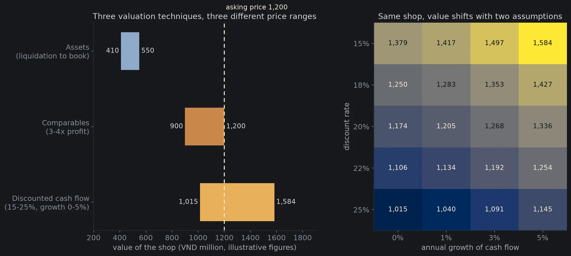
Each technique answers a different question, so there is no reason for them to match:
- Assets answers “how much if everything is sold?”, so it gives the lowest number.
- Comparables answers “what is the market paying for things like it?”.
- Discounted cash flow answers “what is its future worth, under my assumptions?”, so it gives the widest range.
When the three ranges overlap, you have more confidence in the number. When they sit far apart, it is a sign to question the assumptions. In the figure, assets come out far below the other two. That gap is the intangible part: regular customers, location, the owner’s skill.
Three common misunderstandings about valuation
Is a low P/E the same as cheap? Not automatically. A low P/E can mean the market expects profit to fall. Comparison only means something between businesses in the same industry, with the same risk and similar growth prospects. This is my own reasoning from how the ratios are defined, not a measured figure.
Does discounted cash flow give an exact number? No. It is exact mathematically but depends on assumptions. Figure 1 shows that with just two assumptions changed within a reasonable range, the value moves by more than 50%.
Is the market price always the true value? Both Williams and Graham separate the two: price is what people pay today, value is what you estimate about the future[3][4]. When the price is below your estimated value, Graham calls the difference a margin of safety[4]. A margin of safety is a way to survive errors in your own estimate. The articles on the Nash equilibrium and the prisoner’s dilemma explain why other people’s decisions also move prices, even when a business’s value has not changed.
The notation, compactly
This part is for readers who want the formulas. Skipping it does not lose the main idea.
The present value of a payment received years from now, discounted at rate , is
For several payments , add up the present value of each[2]:
When cash flow continues forever and grows steadily at rate , the sum has a compact formula, provided :
For a whole company, the discount rate is usually the weighted average cost of capital (WACC), a blend of the cost of equity and the cost of debt[2]:
where and are the market values of equity and debt, and are their costs, and is the tax rate. The cost of equity is often estimated with the CAPM[2]:
Value a coffee shop yourself
The Python script below values the imaginary coffee shop with all three techniques and draws Figure 1. Every input is illustrative (in VND million): next year’s profit 300, a lease with 8 years left, 100 from reselling equipment at the end of the lease, and assets of 250 for equipment, 100 for furniture and 200 for the deposit. The two softest assumptions in the model are the 3 to 4 times profit multiple of shops in the area and the 60% resale rate of used goods, both set by me. There is no randomness, so no seed is needed. You need numpy and matplotlib.
import matplotlib.pyplot as pltimport numpy as np
plt.rcParams.update({"figure.facecolor": "#16181c", "axes.facecolor": "#16181c", "text.color": "#d4d7dc",                     "axes.edgecolor": "#2a2e35", "axes.labelcolor": "#a4a9b2",                     "xtick.color": "#878d97", "ytick.color": "#878d97", "font.size": 12})
# ILLUSTRATIVE figures for an imaginary coffee shop, in VND million.PROFIT = 300             # cash the owner receives next year (after all costs, including the owner's own pay)YEARS = 8                # the lease has 8 years leftRESALE_AT_END = 100      # what the remaining equipment sells for when the lease endsASKING_PRICE = 1200ASSETS = {"equipment": 250, "furniture": 100, "lease deposit": 200}

def dcf(r, g, n=YEARS):    """Present value of n years of cash flow (growing g per year) plus the resale value, discounted at r."""    years = np.arange(1, n + 1)    cash_flow = PROFIT * (1 + g) ** (years - 1)    return float(np.sum(cash_flow / (1 + r) ** years) + RESALE_AT_END / (1 + r) ** n)

# Technique 1: comparables. Similar shops in the area sell for 3 to 4 times annual profit.comparables = (3 * PROFIT, 4 * PROFIT)
# Technique 3: assets. Upper bound is book value, lower bound is liquidation (equipment and furniture resell at 60%).book_value = sum(ASSETS.values())liquidation = ASSETS["equipment"] * 0.6 + ASSETS["furniture"] * 0.6 + ASSETS["lease deposit"]asset_range = (liquidation, book_value)
# Technique 2: discounted cash flow. Try discount rates of 15% to 25% and growth of 0% to 5%.R = np.array([0.15, 0.18, 0.20, 0.22, 0.25])G = np.array([0.0, 0.01, 0.03, 0.05])grid = np.array([[dcf(r, g) for g in G] for r in R])dcf_range = (grid.min(), grid.max())
print(f"comparables (3-4x profit): {comparables[0]:.0f} - {comparables[1]:.0f}")print(f"assets (liquidation - book): {asset_range[0]:.0f} - {asset_range[1]:.0f}")print(f"DCF base case (r=20%, g=3%): {dcf(0.20, 0.03):.0f}")print(f"DCF range: {dcf_range[0]:.0f} - {dcf_range[1]:.0f}")print(f"discount rate +1 percentage point: {dcf(0.21, 0.03) / dcf(0.20, 0.03) - 1:+.1%}")print(f"growth +1 percentage point: {dcf(0.20, 0.04) / dcf(0.20, 0.03) - 1:+.1%}")

# For comparison: if cash flow lasts forever, the value is CF / (r - g). This formula is far more sensitive.def perpetuity(r, g):    return PROFIT / (r - g)

print(f"perpetuity, r=20%, g=3%: {perpetuity(0.20, 0.03):.0f}; r=21%: {perpetuity(0.21, 0.03) / perpetuity(0.20, 0.03) - 1:+.1%}")print(f"perpetuity, r=10%, g=5%: {perpetuity(0.10, 0.05):.0f}; r=11%: {perpetuity(0.11, 0.05) / perpetuity(0.10, 0.05) - 1:+.1%}")
# Drawfig = plt.figure(figsize=(14, 6.2))o = fig.add_gridspec(1, 2, width_ratios=[1.15, 1], wspace=0.28)
ax = fig.add_subplot(o[0])labels = ["Assets\n(liquidation to book)", "Comparables\n(3-4x profit)", "Discounted cash flow\n(15-25%, growth 0-5%)"]ranges = [asset_range, comparables, dcf_range]colors = ["#8fa9c9", "#c9884a", "#e8b05a"]for i, ((lo, hi), c) in enumerate(zip(ranges, colors)):    ax.barh(i, hi - lo, left=lo, color=c, height=0.5)    ax.text(lo - 15, i, f"{lo:,.0f}", ha="right", va="center", fontsize=11)    ax.text(hi + 15, i, f"{hi:,.0f}", ha="left", va="center", fontsize=11)ax.axvline(ASKING_PRICE, color="#f4e9d2", lw=1.6, ls=(0, (4, 3)))ax.text(ASKING_PRICE + 12, -0.55, f"asking price {ASKING_PRICE:,}", color="#f4e9d2", fontsize=11)ax.set_yticks(range(3))ax.set_yticklabels(labels)ax.invert_yaxis()ax.set_xlim(200, 1900)ax.set_xlabel("value of the shop (VND million, illustrative figures)")ax.set_title("Three valuation techniques, three different price ranges", color="#d4d7dc", fontsize=13)
ax = fig.add_subplot(o[1])ax.imshow(grid, cmap="cividis", aspect="auto")for i in range(len(R)):    for j in range(len(G)):        ax.text(j, i, f"{grid[i, j]:,.0f}", ha="center", va="center", fontsize=11,                color="#16181c" if grid[i, j] > grid.mean() else "#f4e9d2")ax.set_xticks(range(len(G)))ax.set_xticklabels([f"{g:.0%}" for g in G])ax.set_yticks(range(len(R)))ax.set_yticklabels([f"{r:.0%}" for r in R])ax.set_xlabel("annual growth of cash flow")ax.set_ylabel("discount rate")ax.set_title("Same shop, value shifts with two assumptions", color="#d4d7dc", fontsize=13)for a_ in fig.axes:    for sp in ("top", "right"):        a_.spines[sp].set_visible(False)fig.savefig("dinh-gia-quan-ca-phe-en.png", dpi=150, bbox_inches="tight")
Output:
comparables (3-4x profit): 900 - 1200assets (liquidation - book): 410 - 550DCF base case (r=20%, g=3%): 1268DCF range: 1015 - 1584discount rate +1 percentage point: -3.1%growth +1 percentage point: +2.6%perpetuity, r=20%, g=3%: 1765; r=21%: -5.6%perpetuity, r=10%, g=5%: 6000; r=11%: -16.7%The last two lines are the point to notice. With a finite 8-year cash flow, nudging the discount rate by one percentage point changes the value by only about 3%. With a perpetual cash flow, the same nudge changes it by 5.6%, and by as much as 16.7% when the gap between the discount rate and growth is narrow. You can change PROFIT, YEARS or the R and G grids to see how the range moves. A limit of the model: it assumes cash flow is known in advance, while a real shop has busy months and slow ones.
Back to the coffee shop
The three buyers left the shop that Saturday morning with three different numbers, and perhaps all three had calculated correctly. The one who compared had 900 million to 1.2 billion. The one who discounted cash flow had roughly 1 to 1.6 billion. The one who added up assets had 410 to 550 million.
The 1.2 billion asking price sits where two ranges overlap, so none of them found it absurd. But the most careful buyer is the one who asks three more questions: which assumption in my number is the thinnest, if that assumption is off by one percentage point how much does the price change, and am I still willing to pay that price if I am wrong? Valuation is worth doing for how it forces you to name your assumptions, more than for the number it produces.
Free geometry illustrations for students and teachers: EyeViz.
Tài liệu tham khảo
- [1]Valuation (finance). Wikipedia.
- [2]Discounted cash flow. Wikipedia.
- [3]John Burr Williams. Wikipedia.
- [4]Benjamin Graham. Wikipedia.
- [5]John Burr Williams. The Theory of Investment Value. Harvard University Press, 1938.