Base rates and Simpson's paradox: two statistical traps
Why can a 99% accurate test give mostly false positives, and why can success rates reverse when groups are combined? Two statistical traps, explained simply.
Mục lục
You go for a routine health check and receive a report that says “positive” for a rare disease. The doctor says the test is 99% accurate. Most of us would immediately think: so there is a 99% chance I have it.
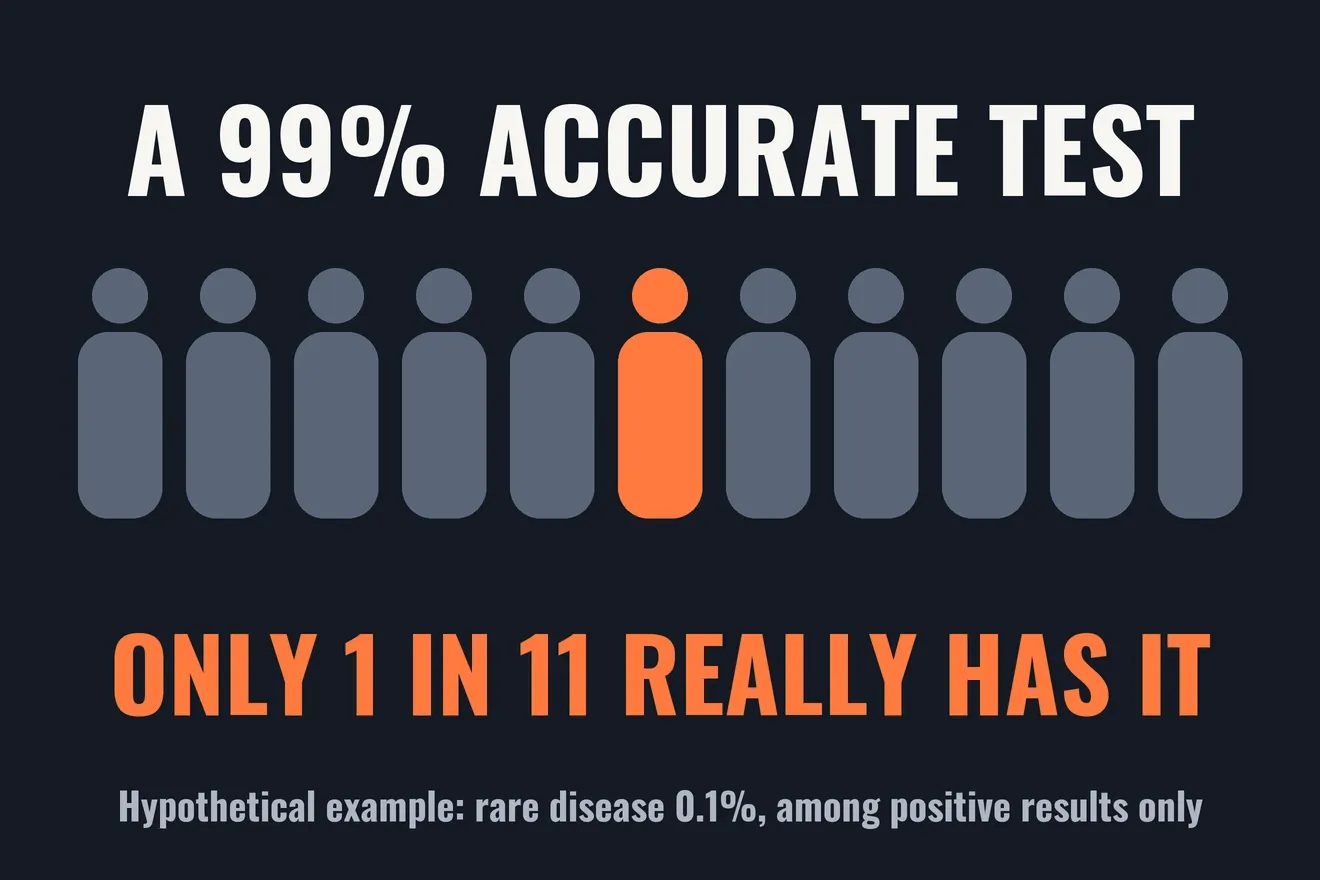
The answer to this medical test problem can be very different. If only 1 person in 1,000 has the disease, then in the hypothetical example below, a positive result corresponds to about a 9% chance of really having it. The test is not bad. The 99% answers one question, while the person holding the report is asking another. The missing piece is the base rate.
The second trap is called Simpson’s paradox: a treatment can have a higher success rate among mild cases and among severe cases, yet a lower one when everyone is combined. This article resolves both traps with a single question: who is this percentage divided by? At the end, the same question is applied to a stock signal using real data.
If a test is 99% accurate, does a positive mean you have the disease?
Picture the anti-theft gate at a supermarket. Out of every 1,000 shoppers, 1 has hidden something in a bag. The gate almost always sounds for that person, but it also sounds by mistake for 1% of ordinary shoppers. Out of 1,000 shoppers, about 10 honest people set it off, against just 1 person hiding something. The alarm is very sensitive, and still most of the people stopped have done nothing wrong.
A medical test works the same way. Let us switch to 100,000 people to make counting easy, and assume three numbers purely for illustration:
- The disease affects 0.1% of people, so 100 have it and 99,900 do not.
- Among those who have it, the test detects 99%.
- Among those who do not, the test correctly reports negative 99% of the time.
| Group of 100,000 people | Positive | Negative | Total |
|---|---|---|---|
| Has the disease | 99 | 1 | 100 |
| Does not have it | 999 | 98,901 | 99,900 |
| Total | 1,098 | 98,902 | 100,000 |
There are 1,098 positive results, but only 99 of those people really have the disease. That is 99 / 1,098, or about 9%. The 99% lives in the two rows of the table, while the person holding the report is standing in the “Positive” column. Rows and columns have different denominators, so they give different answers.
Laying out a table in counts of people like this is called natural frequencies. It is like dividing a pot of sticky rice for a whole neighborhood: counting servings is much easier than adding percentages. Studies show that people reason in a Bayesian way more accurately when information is presented like this[3].
How do sensitivity, specificity and predictive value differ?
These three terms sound alike, but their denominators differ[1][2].
Sensitivity is the share detected among people who really have the disease. At the supermarket gate, it is the percentage of people hiding something who make the gate sound.
Specificity is the share correctly reported negative among people who do not have the disease. At the gate, it is the percentage of ordinary shoppers who pass through in peace.
Positive predictive value (PPV) is the share who really have the disease among people with a positive result. At the gate, it is the percentage of stopped shoppers who really were hiding something. This is the number the person holding the report needs.
Sensitivity and specificity describe the test under the conditions in which it was measured. PPV also depends on the base rate, meaning the chance of having the disease before taking the test. That is why a test has no single PPV that applies to everyone[2]. Forgetting the base rate is a familiar error known as the base rate fallacy[3].
Why does the same test mean different things for different people?
Keep the test the same and change only who is being tested:
| Chance of disease before the test | Positive and really has the disease |
|---|---|
| 0.1% | 9.0% |
| 1% | 50.0% |
| 10% | 91.7% |
| 20% | 96.1% |
| 50% | 99.0% |
When screening a whole healthy community, a rare disease means false positives can outnumber true ones. When someone already has clear symptoms and the doctor is suspicious after an examination, the starting probability is much higher, so the same positive result carries more weight. Trevethan also notes that these measures depend on the test’s threshold and on the people studied, so they should not be treated as fixed properties[1].
This explains why doctors do not just read one line of a report. They ask about symptoms, age and family history, and they often order a confirmatory test. That is how the base rate enters the calculation, even if no formula is written down.
In the example above, someone with a positive result enters a second test with about a 9% chance of having the disease rather than 0.1%. If the second test is also positive, and the errors of the two tests are truly independent, the chance rises to about 90.7%. The word “independent” matters a great deal. Repeating exactly the same test can repeat exactly the same cause of error, so a confirmatory test usually needs a different method of measurement.
You can find the full Bayes formula in the Monty Hall problem (article in Vietnamese). Here we only need a compact form of the counting in the table:
Here is sensitivity, is specificity and is the base rate. The numerator counts true positives. The denominator counts every positive, true and false.
What is Simpson’s paradox?
The first trap comes from misreading a denominator. The second comes from mixing denominators with different compositions.
Imagine two motorbike mechanics in the same neighborhood, with numbers invented for illustration. An takes 90 hard jobs and 10 easy ones. Binh takes 10 hard jobs and 90 easy ones.
| Type of job | An | Binh |
|---|---|---|
| Hard | 54/90 = 60% | 5/10 = 50% |
| Easy | 10/10 = 100% | 81/90 = 90% |
| Combined | 64/100 = 64% | 86/100 = 86% |
For each type of job, An does better. Combined, An falls far behind. No calculation is wrong. An is pulled down by taking most of the hard work, and Binh is lifted up by taking most of the easy work.
That is Simpson’s paradox: a trend appears in each group but disappears or reverses when the groups are combined[5]. Edward Simpson described the phenomenon in a technical paper in 1951[4]. Karl Pearson and Udny Yule had mentioned similar effects earlier, and the name “Simpson’s paradox” was introduced by Colin Blyth in 1972[5].
The hidden variable, in this case how hard the job is, is called a confounder. It affects both who gets the job and how the job turns out. It is like comparing the average scores of two classes while forgetting that one class sat a harder exam.
Simpson’s paradox in kidney stone treatment
In 1986, Charig and colleagues published kidney stone treatment results for 1,052 patients. Open surgery succeeded in 273 of 350 cases, or 78%. Percutaneous stone removal succeeded in 289 of 350, or 83%. Success meant the stones were gone or smaller than 2 mm after three months[7].
Julious and Mullee later used these numbers to illustrate confounding and Simpson’s paradox[8]. Split by stone size, the order reverses[5]:
| Stone size | Open surgery | Percutaneous removal |
|---|---|---|
| Small stones | 81/87 = 93% | 234/270 = 87% |
| Large stones | 192/263 = 73% | 55/80 = 69% |
| Combined | 273/350 = 78% | 289/350 = 83% |
Open surgery received many of the large stones, which are harder. Percutaneous removal received many of the small stones, which are easier. The story is exactly that of the two mechanics.
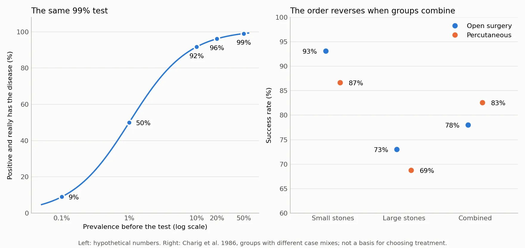
If both methods are put on the same mix of stones, for example the combined mix of all 700 cases, open surgery reaches about 83.3% and percutaneous removal about 77.9%. This calculation only shows that the patient mix created the reversal. It does not conclude which method should be used today. That would take much more data, including complications, cost, recovery time and newer techniques. Charig’s own paper also reports differences in cost and in time to return to normal life across methods[7].
Did Berkeley really discriminate in admissions?
In the fall of 1973, graduate admissions figures at the University of California, Berkeley showed that 44% of men were admitted, compared with 35% of women. The gap was large enough to be unlikely to be due to chance[5]. Looking at the combined number, the natural conclusion was that the university favored men.
Bickel and colleagues examined the data by department[6]. Women tended to apply to more competitive departments, where admission rates were low for everyone. Men tended to apply to departments that were easier to enter. Once department was taken into account, the overall picture did not show the bias in favor of men that the combined figure suggested. Across all 85 departments, 4 showed a significant disadvantage for women and 6 a significant disadvantage for men[5].
The story does not end at “combining is wrong”. The next question remains: why did women concentrate their applications in the departments that were harder to enter? Splitting the statistics moves the question to a better place. It does not make it disappear.
When should you split into groups, and when not?
A common misunderstanding is that splitting into groups is always the safe choice. In fact, choosing which number to trust requires knowing how the variables relate to one another, and the table alone cannot tell you that[5].
Stone size exists before treatment, so it can influence the choice of method. It is a confounder, and splitting by it makes sense.
Now take a different, hypothetical example. A drug lowers blood pressure and thereby reduces complications. If you split patients by their blood pressure after taking the drug, you may erase the very path through which the drug works. It is like asking whether fertilizer helps rice, while comparing only plots with the same plant height at the end of the season. That height is already a result of the fertilizer, so it is no longer a starting condition. In this case the combined number answers the question correctly.
The two examples use the same arithmetic but lead to opposite choices. The difference lies in the causal story: whether the variable used for splitting comes before or after the cause being studied. This is also why randomized controlled trials are valued: random assignment makes the groups alike even on variables nobody has thought of.
Three short questions are worth asking before trusting a percentage:
- Who is the denominator? People with the disease, people who tested positive, or everyone tested?
- What is the base rate? Is this event rare or common?
- Do the groups have the same composition? If not, does the variable that differs come before or after the cause being studied?
The third question is close to survivorship bias (article in Vietnamese): before reading a result, ask how the data in front of you were selected. When comparing before and after an action, the article on regression to the mean (article in Vietnamese) covers another trap that can appear at the same time.
Is a stock signal like a positive test result?
An investment signal resembles a medical test. The “disease” is the event we want to predict, and a “positive” is a day when the signal appears. I tested this on FPT’s closing prices from January 2020 to December 2025, with a rule fixed before looking at the results and with no variations tried:
- Signal: today’s close is above the highest close of the previous 20 sessions.
- Event: exactly 20 sessions later, the close is at least 10% above today’s close.
Across 1,479 measurable sessions, the event occurred in 229, giving a base rate of 15.5%. The signal appeared 221 times, and the event followed in 35 of them.
| Year | Signal count | Event rate with signal | Event rate without signal |
|---|---|---|---|
| 2020 | 35 | 14.3% | 19.4% |
| 2021 | 41 | 26.8% | 17.2% |
| 2022 | 28 | 17.9% | 11.8% |
| 2023 | 46 | 8.7% | 12.8% |
| 2024 | 54 | 18.5% | 28.1% |
| 2025 | 17 | 0.0% | 4.2% |
| Combined | 221 | 15.8% | 15.4% |
The 15.8% is almost identical to the base rate. The signal appeared in 15.3% of sessions with the event and 14.9% of sessions without it. When those two rates are nearly equal, a “positive” barely changes what we should believe, just like a test that sounds about equally for sick and healthy people.
The yearly table shows one more thing. Over the six years combined, days with the signal come out 0.4 percentage points ahead. But the signal does worse in four of the six years, and averaging the yearly differences by number of sessions puts it about 1.2 percentage points behind. This is not a complete Simpson’s paradox, because 2021 and 2022 go the other way. It only shows the same mechanism on a small scale: the signal appeared often in 2024, a year with a high base rate, which lifted the combined number. On this data, the honest statement is that the signal shows no clear edge.
Run it yourself: drawing the two statistical traps
The Python below needs only matplotlib. It computes the predictive value table and the kidney stone table, and produces exactly Figure 1. There is no randomness, so it gives the same result every time.
import matplotlib.pyplot as plt
# Part 1: a hypothetical test, 99% sensitivity, 99% specificitydef ppv(prevalence, sens=0.99, spec=0.99):    true_pos = sens * prevalence    false_pos = (1 - spec) * (1 - prevalence)    return true_pos / (true_pos + false_pos)
marks = [0.001, 0.01, 0.1, 0.2, 0.5]for p in marks:    print(f"Prevalence {p:6.1%} -> positive and really has it {ppv(p):6.1%}")print(f"Independent second test: {ppv(ppv(0.001)):.1%}")
# Part 2: the kidney stone table, (successes, cases)data = {"Open surgery": {"Small stones": (81, 87), "Large stones": (192, 263)},        "Percutaneous": {"Small stones": (234, 270), "Large stones": (55, 80)}}groups = ["Small stones", "Large stones"]size = {g: sum(data[t][g][1] for t in data) for g in groups}total = sum(size.values())rates = {}for t, row in data.items():    wins = sum(a for a, _ in row.values())    cases = sum(b for _, b in row.values())    fixed_mix = sum(row[g][0] / row[g][1] * size[g] / total for g in groups)    rates[t] = [row[g][0] / row[g][1] for g in groups] + [wins / cases]    print(f"{t}: combined {wins}/{cases} = {wins / cases:.1%}, same mix = {fixed_mix:.1%}")
# Part 3: two panels, one question each, no dual axisfig, (left, right) = plt.subplots(1, 2, figsize=(11, 5.2), dpi=160, facecolor="#fcfcfb")xs = [0.0005 * 1.05 ** i for i in range(146)]left.semilogx(xs, [ppv(x) * 100 for x in xs], color="#2a78d6", lw=2)for p in marks:    y = ppv(p) * 100    left.plot(p, y, "o", color="#2a78d6", ms=8, mec="#fcfcfb", mew=2)    left.annotate(f"{y:.0f}%", (p, y), (0, -17) if p >= 0.1 else (10, -4),                  textcoords="offset points", ha="center" if p >= 0.1 else "left", fontsize=10)left.set_xticks(marks, ["0.1%", "1%", "10%", "20%", "50%"])left.minorticks_off()left.set_ylim(0, 108)left.set_xlabel("Prevalence before the test (log scale)")left.set_ylabel("Positive and really has the disease (%)")left.set_title("The same 99% test", loc="left", fontsize=12)
names = ["Small stones", "Large stones", "Combined"]for t, color, offset in [("Open surgery", "#2a78d6", -0.1), ("Percutaneous", "#eb6834", 0.1)]:    ys = [r * 100 for r in rates[t]]    right.plot([i + offset for i in range(3)], ys, "o", color=color, ms=10,               mec="#fcfcfb", mew=2, label=t)    for i, y in enumerate(ys):        right.annotate(f"{y:.0f}%", (i + offset, y), (-24 if offset < 0 else 24, -4),                       textcoords="offset points", ha="center", fontsize=10)right.set_xticks(range(3), names)right.set_xlim(-0.6, 2.6)right.set_ylim(60, 100)right.set_ylabel("Success rate (%)")right.set_title("The order reverses when groups combine", loc="left", fontsize=12)right.legend(frameon=False, loc="upper right")
for ax in (left, right):    ax.set_facecolor("#fcfcfb")    ax.grid(axis="y", color="#e4e3df", lw=0.8)    ax.spines[["top", "right"]].set_visible(False)    ax.spines[["left", "bottom"]].set_color("#b8b7b0")    ax.tick_params(colors="#52514e", length=0)fig.text(0.5, 0.012, "Left: hypothetical numbers. Right: Charig et al. 1986, groups with different case mixes; not a basis for choosing treatment.",         ha="center", color="#52514e", fontsize=9)fig.tight_layout(rect=(0, 0.04, 1, 1))fig.savefig("bay-ti-le-en.png", facecolor="#fcfcfb")
Prevalence 0.1% -> positive and really has it 9.0%Prevalence 1.0% -> positive and really has it 50.0%Prevalence 10.0% -> positive and really has it 91.7%Prevalence 20.0% -> positive and really has it 96.1%Prevalence 50.0% -> positive and really has it 99.0%Independent second test: 90.7%Open surgery: combined 273/350 = 78.0%, same mix = 83.3%Percutaneous: combined 289/350 = 82.6%, same mix = 77.9%Try changing specificity from 0.99 to 0.999 while keeping prevalence at 0.1%. The positive predictive value rises to about 50%, even though specificity moved by less than one percentage point. For a rare disease, the number of false positives is what decides the outcome.
Back to the test report
The report saying “positive” and the number 99% are both correct. What is missing is one question: 99% of whom? For a rare disease and a person with no symptoms, the group standing beside you includes many healthy people with false positives. That is why the next step is a confirmatory test, not a conclusion of your own.
Mechanic An, the patients with large stones and the hard-to-enter Berkeley departments show the same thing from the opposite direction. A combined rate can reflect who was placed in which group more than it reflects the quality of what is being measured.
Before you trust a percentage, read its denominator.
Free geometry illustrations for students and teachers: EyeViz.
Tài liệu tham khảo
- [1]Robert Trevethan. Sensitivity, Specificity, and Predictive Values: Foundations, Pliabilities, and Pitfalls in Research and Practice. Frontiers in Public Health, 5, 307, 2017.
- [2]Positive and negative predictive values. Wikipedia, 2026.
- [3]Base rate fallacy. Wikipedia, 2026.
- [4]Edward H. Simpson. The Interpretation of Interaction in Contingency Tables. Journal of the Royal Statistical Society, Series B, 13(2), 238–241, 1951.
- [5]Simpson's paradox. Wikipedia, 2026.
- [6]P. J. Bickel, E. A. Hammel, J. W. O'Connell. Sex Bias in Graduate Admissions: Data from Berkeley. Science, 187(4175), 398–404, 1975.
- [7]C. R. Charig, D. R. Webb, S. R. Payne, J. E. Wickham. Comparison of treatment of renal calculi by open surgery, percutaneous nephrolithotomy, and extracorporeal shockwave lithotripsy. British Medical Journal, 292(6524), 879–882, 1986.
- [8]Steven A. Julious, Mark A. Mullee. Confounding and Simpson's paradox. BMJ, 309(6967), 1480–1481, 1994.