Why is the sum of the two roots always −b/a? Viète and what the parabola shows
Why does the sum of the roots equal −b/a? Viète’s theorem on a parabola: the HUST Parabol Gate, artillery shells, a thrown ball and computers.
Mục lục
Why is the sum of the roots always −b/a?
In grade 9 you learn a shortcut: the equation has two roots, and without solving it you already know their sum is 5 and their product is 6. The sum is and the product is . This is Viète’s theorem[1][3]. Check it: the roots are 2 and 3, the sum is 5, the product is 6.
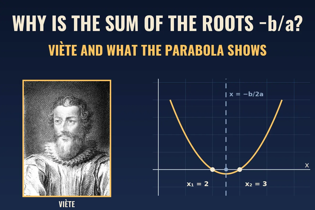
The short answer to “why”: the graph of is a parabola, and a parabola is symmetric about a vertical line [[4]]. The two roots are the two points where the parabola crosses the x axis, so they are equally far from that line. The midpoint of the roots is , which means their sum is . The product can be read off by rewriting .
This article covers four things. What the theorem says and how to use it, how the parabola shows why it is true (with the Parabol Gate of Hanoi University of Science and Technology), who Viète was and why the theorem carries his name (the story is less tidy than the name). Then the places where the theorem is at work: a ball thrown into the air, the two firing angles of artillery, the small root that computers often get wrong, and matrices.
What does Viète’s theorem say, and how do you use it?
For an equation with two roots and (counting a double root twice), there are two relations:
Picture a rectangular garden with a perimeter of 14 meters and an area of 12 square meters. Half the perimeter is 7, so the two sides add up to 7. The area is 12, so the two sides multiply to 12. The sides are the roots of . You do not need the quadratic formula: just find two numbers with sum 7 and product 12, which are 3 and 4.
It also works backwards. To get an equation with roots 2 and 3, take the sum 5 and the product 6 and write . And after solving a quadratic you can check your answer with these two relations, the way you check a division by multiplying.
Why is it true? Look at the parabola
Fold a sheet of paper with a parabola drawn on it along the parabola’s axis of symmetry. The two branches land on top of each other, and so do the two points where it meets the x axis. The axis of is at [[4]]. The two roots are equally far from it, so one root sits at and the other at for the same offset . Add them and the offsets cancel, leaving .
The quadratic formula says exactly this. It writes the roots as [[3]]: the position of the axis, , plus or minus an offset . The source also notes that the x coordinate of the vertex is at the average of the roots[[3]].
And the product? If and are the roots, then is a parabola with the same and the same two crossing points, so it is the original parabola. Expanding:
Comparing with gives and . Both relations appear at once. The picture also gives a reading of : it is the height where the parabola crosses the y axis, and it equals times the product of the roots.
What if the parabola does not reach the x axis? Then and the two roots are complex conjugates[[3]]. Both relations still hold. For example has roots and : the sum is 0, which is with , and the product is 1, which is . Figure 5 in the code section draws this very parabola, , with its axis and its two roots.
The Parabol Gate of Bách khoa: the two feet of the gate are the two roots
If you have studied at or walked past the Hanoi University of Science and Technology (Bách khoa), you know the Parabol Gate. According to VOV, the gate was built more than 50 years ago, and its name comes from a curved arch design that recalls the graph of a parabola[[8]]. The article, published on 3 November 2026, says the university will set the gate back about 20 meters, tied to site clearance for the Route 1A “space axis” project, and that the gate will be kept as a landmark[[8]].
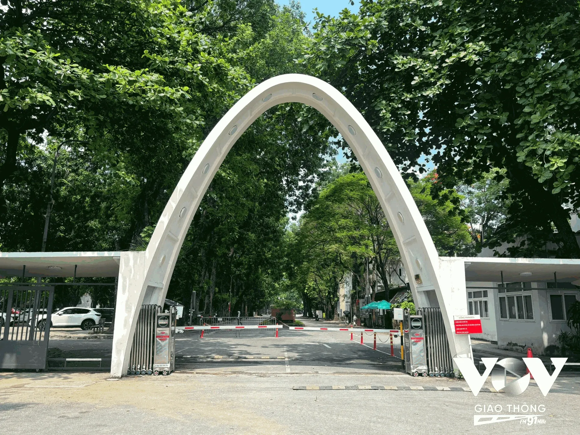
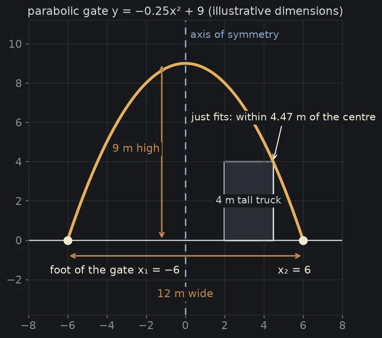
I could not find the real dimensions of the gate, so the numbers below are illustrative. Put the origin at the middle of the two feet, with meters as the unit, and treat the arch as the parabola : 9 meters high at the centre. The feet of the gate are where , the two roots of , which are and . Viète’s theorem gives two facts almost at once. The sum of the roots is (because ): the two feet are equally far from the centre line of the gate. The product is .
The width of the gate is the difference of the roots. From the quadratic formula that difference is meters. With an arch like this, a 4-meter-tall truck fits only while it stays within meters of the centre line, because gives . Figure 2 redraws the gate with those numbers, together with the truck that just fits.
A ball thrown upward: Viète’s theorem in physics
Galileo showed that the path of a thrown object is a parabola, and the principle of compound motion he established in 1638 was what he used to prove it[[4]][[5]]. The article Galileo: And Yet It Moves tells more about the years when he wrote that book.
Ignoring air resistance, the height of a ball thrown straight up with initial speed is [[5]]. Imagine you throw a ball up at m/s with m/s² (illustrative numbers). When it passes the height m, the ball is there twice: once on the way up and once on the way down, like someone passing a second-floor window on the way up and again on the way down the stairs.
Setting gives , a quadratic in time. Viète’s theorem gives two facts without solving it:
- The sum of the two times is seconds, which is exactly the whole flight time. The reason is that the two moments are symmetric around the instant the ball reaches its peak, and the peak sits exactly halfway through the flight[[5]].
- The product of the two times is seconds squared.
The code section computes the actual roots: the ball is at 3 m at 0.365 seconds and at 1.675 seconds. The sum is 2.041 and the product is 0.612, as predicted.
Artillery: two firing angles, one range
For a long time artillery had to answer a practical question: at what angle should you fire to make the shell go farthest? In 1537 Niccolò Tartaglia published Nova Scientia, and according to his biography he held that the maximum range is reached when the barrel points 45 degrees above the horizontal[[9]]. But he pictured the shell flying straight, then bending along a circular arc, then dropping straight down[[9]], not along a parabola. The parabola came later, from Galileo in 1638[[5]].
Ignoring air resistance, a shell fired from the ground with speed at angle travels , which is largest at 45 degrees[[5]]. Suppose you must hit a target 800 meters away at the same height as the gun, with a shell speed of 100 m/s (illustrative numbers). There are two ways to fire. A low shot makes the shell fly fast and almost straight. A high shot sends it up and lets it fall almost straight down, like a high arcing throw into a basket compared with a flat throw. The source also gives two solutions for the angle, a low one and a high one[[5]].
Viète tells you how those two angles are related without solving anything. The path is . Setting at and dividing both sides by gives a quadratic in :
The product of the roots is , that is . Two angles whose tangents multiply to 1 are complementary: . So the high shot and the low shot always come as a pair that adds up to 90 degrees. With the numbers above, the code gives 25.8° and 64.2°, summing to exactly 90°, and checks that both land at 800 meters (Figure 3).
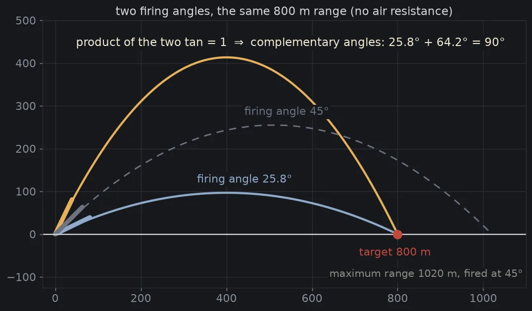
The sum of the roots tells one more thing. The sum is . As grows the sum shrinks, the two roots move together, and they coincide when the sum equals 2, that is , where both angles are 45 degrees. That is exactly the maximum range, 1,020 meters for m/s. Farther than that : the equation has no real root, and no angle can send the shell that far.
The limits need to be stated. A real shell also feels air resistance, a force that always points against the direction of motion[[5]], so the real path departs from a parabola. The numbers above hold only when air resistance is ignored.
Who was Viète, and why does the theorem carry his name?
François Viète was born in 1540 in Fontenay-le-Comte (France) and died on 23 February 1603 in Paris. He was a lawyer and a counselor to King Henry III and then Henry IV[[2]]. In 1590 he broke a Spanish cipher of more than 500 characters. The source says the King of Spain later accused him of using magical powers[[2]].
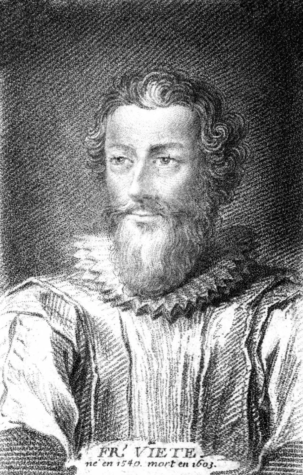
The contribution that matters for this article is a change in how equations are written. In 1591 he published In artem analyticem isagoge, where he used letters: consonants for known quantities and vowels for unknowns[[2]]. Before that, equations were usually stated in words or worked with specific numbers, one solution per problem. Letters let you say something once for all equations. It is like a spreadsheet: instead of writing a ready-made sum of 3 and 4, you write “cell A1 plus cell B1” and fill in the numbers later. Without letters , , standing for the coefficients, nobody could state “the sum of the roots is ” for every quadratic. One could only give examples.
The naming you learned at school, with the unknown, comes from a later step. In 1637 Descartes used the last letters of the alphabet (, , ) for unknown quantities and the first letters (, , ) for known ones[[7]]. The article Why do we need the x and y axes? is about that book, La Géométrie.
And the link between roots and coefficients? The source says Viète established it for the case of positive roots[[1]][[2]]. According to Charles Hutton, an 18th-century English mathematician quoted by the source, the first person to understand the general principle, not limited to positive roots, was Albert Girard, a 17th-century French mathematician[[1]]. The source also remarks that Viète’s methods were very close to those of the 12th-century Islamic mathematician Sharaf al-Din al-Tusi[[1]]. So “Viète’s theorem” is a name by habit, not evidence that he alone found everything.
It also helps to place the theorem in the longer history of the quadratic. Babylonian mathematicians recorded problems leading to it on clay tablets around 2000 BC. In 628, Brahmagupta gave the first explicit solution, not yet fully general. In the 9th century al-Khwarizmi gave a complete solution. In 1594 Simon Stevin had a formula covering all cases, and in 1637 Descartes published it in its modern form[[3]]. Viète sits in the middle of that line, with letters and with relations between roots and coefficients.
One last correction. Viète did not draw a parabola to prove anything. Descartes’ coordinates appeared in La Géométrie in 1637, more than forty years after Viète’s Isagoge[[2]][[7]]. The view “the two roots are equally far from the axis of symmetry” is an explanation that later generations gained from graphs, not the way Viète worked.
If the theorem did not exist, what could not exist?
A relation between two roots and three coefficients sounds small. Here are three places where it works, from your phone to statistics.
Computers: finding the small root without losing digits
The quadratic formula has a weak spot. When is much larger than , the numbers and are nearly equal, and subtracting them destroys most of the significant digits. The source calls this loss of significance (catastrophic cancellation) in the smaller root[[3]]. The way around it is to compute the larger root first, by an addition, and then take the smaller root as [[3]]. That is Viète’s product relation.
Imagine you want the thickness of one sheet of paper. You measure a stack of 500 sheets, measure a stack of 499 sheets with a poor ruler, and subtract. Two large numbers are nearly equal, so the thickness you want is buried in the ruler’s error. Dividing the height of the stack by 500 avoids that subtraction.
I tried it on , whose small root is about . With 64-bit floating point and , the quadratic formula gives instead of , an error of about 25.5%. With it gives 0. The Viète approach gives exactly and in both cases (my own run, in the code section below; the reference is a 60-digit decimal calculation).
Matrices: sum and product of eigenvalues
A matrix has two eigenvalues, the two numbers that say how much the matrix stretches its special directions. They are the roots of a quadratic in . Viète’s theorem says the sum of the two eigenvalues equals the trace of the matrix (the sum of the two diagonal entries) and their product equals the determinant. The source states this for every size: the trace is the sum of the eigenvalues and the determinant is their product[[6]]. For example, the matrix has characteristic equation , so its eigenvalues are 1 and 3, the sum 4 equals the trace and the product 3 equals the determinant[[6]].
This is used in statistics. For a covariance matrix, the eigenvalues correspond to the variance explained by each principal component[[6]]. It follows from the theorem that the sum of those variances equals the trace of the matrix, the total variance of the original variables. It is like slicing a cake: however you cut it, the pieces add up to the whole cake.
A quadratic is the model problem for optimization
When teaching a computer to find the lowest point of a function, people often test on a parabola, because we know where the answer is: the bottom is at . The article Gradient descent uses exactly the model to show how small or large steps make the algorithm slow or make it overshoot.
Four common misunderstandings
Did Viète find the theorem by himself? Not quite. The source says he established it for positive roots, Albert Girard is credited with understanding the general principle, and Viète’s methods were very close to those of Sharaf al-Din al-Tusi before him[[1]].
Do you have to solve the equation before you know the sum and product? The other way round: the sum and product are read straight from the three coefficients without solving. That is why the theorem is useful when roots are hard to compute or when you want to check an answer.
If the parabola does not meet the x axis, are the relations false? No. Then the roots are complex conjugates[[3]], and the sum is still and the product still . The difference is that the roots are no longer real crossing points of the parabola with the x axis.
Is a real artillery shell’s path a parabola? Only if air resistance is ignored. The parabola is Galileo’s result for motion under gravity alone[[5]]. In reality drag bends the path away from it, so numbers like the pair of complementary angles in the artillery section belong to an idealized model, not to the firing table of a real gun.
The notation, compactly
This part is for readers who want the formulas. Skipping it loses nothing essential.
For the quadratic with :
For the cubic with roots [[1]]:
For a polynomial of degree , , the sum of the roots is and the product of the roots is [[1]]. The stable way to compute the small root from the previous section is, with the root of larger absolute value:
Run it yourself: the parabola, the gun, the gate and the accuracy of a root
The Python script below does five things and draws three figures: two for the sections above (the gate and the shell paths) and figure 5 below. It checks both Viète relations on , solves the ball problem at a height of 3 meters and the two firing angles of the gun. Then it computes the parabolic gate with illustrative dimensions, and compares two ways of computing the small root of as grows from 10 to . There is no randomness, so you get the same result every run. At the quadratic formula returns exactly 0.
import mathfrom decimal import Decimal, getcontextimport numpy as npimport matplotlib.pyplot as plt
plt.rcParams.update({"figure.facecolor": "#16181c", "axes.facecolor": "#16181c", "text.color": "#d4d7dc",                     "axes.edgecolor": "#2a2e35", "axes.labelcolor": "#a4a9b2",                     "xtick.color": "#878d97", "ytick.color": "#878d97", "font.size": 12})
# Part 1: x² − 5x + 6 = 0. Hai nghiệm đối xứng qua trục x = −b/2a, nên tổng = −b/a, tích = c/a.a, b, c = 1, -5, 6d = b * b - 4 * a * cx1, x2 = (-b - math.sqrt(d)) / (2 * a), (-b + math.sqrt(d)) / (2 * a)axis = -b / (2 * a)print(f"roots: {x1:g} and {x2:g}; axis of symmetry x = {axis:g}")print(f"sum = {x1 + x2:g} (−b/a = {-b / a:g}); product = {x1 * x2:g} (c/a = {c / a:g})")
# Part 2: a ball thrown up at v0 = 10 m/s (no air resistance). At h = 3 m the ball passes twice.g, v0, h = 9.8, 10.0, 3.0# h = v0·t − g·t²/2  ⇔  t² − (2v0/g)·t + 2h/g = 0tb, tc = -2 * v0 / g, 2 * h / gtd = tb * tb - 4 * tct1, t2 = (-tb - math.sqrt(td)) / 2, (-tb + math.sqrt(td)) / 2print(f"the ball is at {h:g} m at t = {t1:.3f} s and {t2:.3f} s; sum = {t1 + t2:.3f} s (flight time 2·v0/g = {2 * v0 / g:.3f} s); product = {t1 * t2:.3f} (2h/g = {2 * h / g:.3f})")
# Part 4: a gun firing from the ground at a target at the same height, v0 = 100 m/s, d = 800 m away (no air resistance).# y = x·tanθ − g·x²(1 + tan²θ) / (2v²) = 0 ⇒ t² − (2v²/(g·d))·t + 1 = 0 with t = tanθ: the product of the roots is 1.V, D = 100.0, 800.0s = 2 * V ** 2 / (g * D)t1, t2 = (s + math.sqrt(s * s - 4)) / 2, (s - math.sqrt(s * s - 4)) / 2th1, th2 = math.degrees(math.atan(t1)), math.degrees(math.atan(t2))R1, R2 = V ** 2 * math.sin(2 * math.radians(th1)) / g, V ** 2 * math.sin(2 * math.radians(th2)) / gprint(f"gun: sum of tan = {t1 + t2:.3f} (2v²/(g·d) = {2 * V ** 2 / (g * D):.3f}); product of tan = {t1 * t2:.3f}")print(f"two firing angles: {th1:.1f}° and {th2:.1f}° (sum {th1 + th2:.1f}°); range check: {R1:.0f} m and {R2:.0f} m")print(f"maximum range v²/g = {V ** 2 / g:.0f} m, reached at 45°")
# Part 5: a parabolic gate, illustrative dimensions (not real ones): y = −0.25x² + 9, the feet of the gate at the two roots.ga, gb, gc = -0.25, 0.0, 9.0gd = gb * gb - 4 * ga * gcxa, xb = sorted([(-gb + math.sqrt(gd)) / (2 * ga), (-gb - math.sqrt(gd)) / (2 * ga)])half = math.sqrt((gc - 4) / -ga)print(f"a 4 m tall truck fits when it stays within {half:.2f} m of the gate centre")print(f"gate: roots {xa:g} and {xb:g}; sum = {xa + xb:g} (−b/a = {-gb / ga:g}); product = {xa * xb:g} (c/a = {gc / ga:g}); width = {math.sqrt(gd) / abs(ga):g} m")
getcontext().prec = 60# Part 3: small root of x² − B·x + 1 = 0 for huge B. The true root is about 1/B.def naive(B):    # quadratic formula: subtracts two nearly equal numbers    return (B - math.sqrt(B * B - 4)) / 2
def viete(B):    # larger root R first (an addition, no lost digits), then small root = (c/a) / R by Viète's theorem    R = (B + math.sqrt(B * B - 4)) / 2    return 1.0 / R
Bs = 10.0 ** np.arange(1, 9.01, 0.25)err_n, err_v = [], []for B in Bs:    # reference: 60-digit decimals    Bd = Decimal(float(B))    ref = float((Bd - (Bd * Bd - 4).sqrt()) / 2)    err_n.append(max(abs(naive(B) - ref) / ref, 1e-17))    err_v.append(max(abs(viete(B) - ref) / ref, 1e-17))B = 1e8Bd = Decimal(B)ref = float((Bd - (Bd * Bd - 4).sqrt()) / 2)print(f"B = 1e8: reference small root {ref:.6e}; quadratic formula {naive(B):.6e} (error {abs(naive(B) - ref) / ref:.1%}); with Viète {viete(B):.6e} (error below {max(abs(viete(B) - ref) / ref, 1e-16):.0e})")
B = 1e9print(f"B = 1e9: the quadratic formula gives {naive(B):.1e}, with Viète {viete(B):.6e}")
# Drawfig, (ax1, ax2) = plt.subplots(1, 2, figsize=(14, 6.2), gridspec_kw={"wspace": 0.22})xs = np.linspace(0.6, 4.4, 300)ax1.plot(xs, a * xs ** 2 + b * xs + c, color="#e8b05a", lw=2.6)ax1.axhline(0, color="#d4d7dc", lw=1.3)ax1.axvline(axis, color="#8fa9c9", lw=1.8, ls=(0, (5, 4)))ax1.scatter([x1, x2], [0, 0], color="#f4e9d2", s=80, zorder=4)ax1.scatter([axis], [0], color="#8fa9c9", s=60, zorder=4)ax1.annotate(f"x₁ = {x1:g}", (x1, 0), xytext=(x1 - 0.62, -0.62), color="#f4e9d2", fontsize=12.5)ax1.annotate(f"x₂ = {x2:g}", (x2, 0), xytext=(x2 + 0.12, -0.62), color="#f4e9d2", fontsize=12.5)ax1.annotate("axis x = −b/2a = 2.5", (axis, 0), xytext=(axis + 0.1, 2.2), color="#8fa9c9", fontsize=12.5)ax1.annotate("", xy=(x1, -0.35), xytext=(axis, -0.35), arrowprops=dict(arrowstyle="<->", color="#c9884a", lw=1.6))ax1.annotate("", xy=(x2, -0.35), xytext=(axis, -0.35), arrowprops=dict(arrowstyle="<->", color="#c9884a", lw=1.6))ax1.text(axis, -1.02, "both roots equally far from the axis", color="#c9884a", ha="center", fontsize=12, bbox=dict(facecolor="#16181c", edgecolor="none", pad=2))ax1.scatter([0], [c], color="#c9884a", s=0)ax1.set_xlim(0.6, 4.4); ax1.set_ylim(-1.3, 3.4)ax1.set_title("y = x² − 5x + 6: sum 2 + 3 = 5, product 2·3 = 6", color="#d4d7dc", fontsize=13)ax1.grid(color="#2a2e35", lw=0.8)
ax2.loglog(Bs, err_n, color="#c4483d", lw=2.4, label="quadratic formula (subtracts two close numbers)")ax2.loglog(Bs, err_v, color="#e8b05a", lw=2.4, label="larger root first, then (c/a) divided by it (Viète)")ax2.set_xlabel("B in x² − B·x + 1 = 0")ax2.set_ylabel("relative error of the small root")ax2.set_title("Small root in 64-bit floating point", color="#d4d7dc", fontsize=13)ax2.legend(facecolor="#16181c", edgecolor="#2a2e35", fontsize=11, loc="center left")ax2.grid(color="#2a2e35", lw=0.8, which="both")fig.savefig("viete-parabol-en.png", dpi=130, bbox_inches="tight")
# Hình A: hai đường đạn cùng tầm xafig2, bx1 = plt.subplots(figsize=(10, 5.4))for th, col, lab in ((th2, "#8fa9c9", f"{th2:.1f}°"), (th1, "#e8b05a", f"{th1:.1f}°"), (45.0, "#6b7280", "45°")):    x = np.linspace(0, V ** 2 * math.sin(2 * math.radians(th)) / g, 300)    y = x * math.tan(math.radians(th)) - g * x ** 2 / (2 * V ** 2 * math.cos(math.radians(th)) ** 2)    bx1.plot(x, y, color=col, lw=2.4 if th != 45.0 else 1.6, ls="-" if th != 45.0 else (0, (5, 4)))    bx1.annotate(f"firing angle {lab}", (x[len(x) // 2], y[len(x) // 2]), xytext=(x[len(x) // 2] - 70, y[len(x) // 2] + 24), color=col, fontsize=12, bbox=dict(facecolor="#16181c", edgecolor="none", pad=2))    # nòng pháo: một đoạn ngắn theo hướng bắn    bx1.plot([0, 90 * math.cos(math.radians(th))], [0, 90 * math.sin(math.radians(th))], color=col, lw=5, solid_capstyle="round")bx1.axhline(0, color="#d4d7dc", lw=1.3)bx1.scatter([D], [0], color="#c4483d", s=90, zorder=5)bx1.annotate("target 800 m", (D, 0), xytext=(D - 90, -50), color="#c4483d", fontsize=12, bbox=dict(facecolor="#16181c", edgecolor="none", pad=2))bx1.annotate(f"maximum range {V ** 2 / g:.0f} m, fired at 45°", (V ** 2 / g, 0), xytext=(V ** 2 / g - 380, -100), color="#8e8b84", fontsize=11.5, bbox=dict(facecolor="#16181c", edgecolor="none", pad=2))bx1.text(550, 440, "product of the two tan = 1  ⇒  complementary angles: 25.8° + 64.2° = 90°", color="#f4e9d2", ha="center", fontsize=12.5, bbox=dict(facecolor="#16181c", edgecolor="none", pad=2))bx1.set_xlim(-30, 1100); bx1.set_ylim(-125, 500); bx1.set_aspect("equal")bx1.set_title("two firing angles, the same 800 m range (no air resistance)", color="#d4d7dc", fontsize=13)bx1.grid(color="#2a2e35", lw=0.8)fig2.savefig("viete-phao-en.png", dpi=130, bbox_inches="tight")
# Hình B: cổng parabol với chiếc xe cao 4 mfig3, bx2 = plt.subplots(figsize=(8, 6))gx = np.linspace(xa, xb, 200)bx2.plot(gx, ga * gx ** 2 + gb * gx + gc, color="#e8b05a", lw=3.2)bx2.axhline(0, color="#d4d7dc", lw=1.3)bx2.axvline(0, color="#8fa9c9", lw=1.6, ls=(0, (5, 4)))bx2.text(0.25, 10.3, "axis of symmetry", color="#8fa9c9", fontsize=11.5, bbox=dict(facecolor="#16181c", edgecolor="none", pad=2))bx2.scatter([xa, xb], [0, 0], color="#f4e9d2", s=80, zorder=4)bx2.annotate("foot of the gate x₁ = −6", (xa, 0), xytext=(xa - 0.9, -1.7), color="#f4e9d2", fontsize=12, bbox=dict(facecolor="#16181c", edgecolor="none", pad=2))bx2.annotate("x₂ = 6", (xb, 0), xytext=(xb - 1.3, -1.7), color="#f4e9d2", fontsize=12, bbox=dict(facecolor="#16181c", edgecolor="none", pad=2))bx2.annotate("", xy=(xa, -0.8), xytext=(xb, -0.8), arrowprops=dict(arrowstyle="<->", color="#c9884a", lw=1.6))bx2.text(0, -2.9, "12 m wide", color="#c9884a", ha="center", fontsize=12, bbox=dict(facecolor="#16181c", edgecolor="none", pad=2))bx2.annotate("", xy=(-1.2, 9), xytext=(-1.2, 0), arrowprops=dict(arrowstyle="<->", color="#c9884a", lw=1.6))bx2.text(-1.3, 4.5, "9 m high", color="#c9884a", ha="right", fontsize=12, bbox=dict(facecolor="#16181c", edgecolor="none", pad=2))tw = 2.5bx2.add_patch(plt.Rectangle((half - tw, 0), tw, 4, facecolor="#2a2e35", edgecolor="#d4d7dc", lw=1.6))bx2.text(half - tw / 2, 2.0, "4 m tall truck", color="#d4d7dc", ha="center", va="center", fontsize=11, bbox=dict(facecolor="#16181c", edgecolor="none", pad=2))bx2.annotate("just fits: within 4.47 m of the centre", (half, 4), xytext=(0.3, 6.1), color="#f4e9d2", fontsize=11.5, arrowprops=dict(arrowstyle="->", color="#f4e9d2", lw=1.2), bbox=dict(facecolor="#16181c", edgecolor="none", pad=2))bx2.set_xlim(-8, 8); bx2.set_ylim(-3.8, 11.2); bx2.set_aspect("equal")bx2.set_title("parabolic gate y = −0.25x² + 9 (illustrative dimensions)", color="#d4d7dc", fontsize=13)bx2.grid(color="#2a2e35", lw=0.8)fig3.savefig("viete-cong-en.png", dpi=130, bbox_inches="tight")
The output when I ran it:
roots: 2 and 3; axis of symmetry x = 2.5sum = 5 (−b/a = 5); product = 6 (c/a = 6)the ball is at 3 m at t = 0.365 s and 1.675 s; sum = 2.041 s (flight time 2·v0/g = 2.041 s); product = 0.612 (2h/g = 0.612)gun: sum of tan = 2.551 (2v²/(g·d) = 2.551); product of tan = 1.000two firing angles: 64.2° and 25.8° (sum 90.0°); range check: 800 m and 800 mmaximum range v²/g = 1020 m, reached at 45°a 4 m tall truck fits when it stays within 4.47 m of the gate centregate: roots -6 and 6; sum = 0 (−b/a = 0); product = -36 (c/a = -36); width = 12 mB = 1e8: reference small root 1.000000e-08; quadratic formula 7.450581e-09 (error 25.5%); with Viète 1.000000e-08 (error below 1e-16)B = 1e9: the quadratic formula gives 0.0e+00, with Viète 1.000000e-09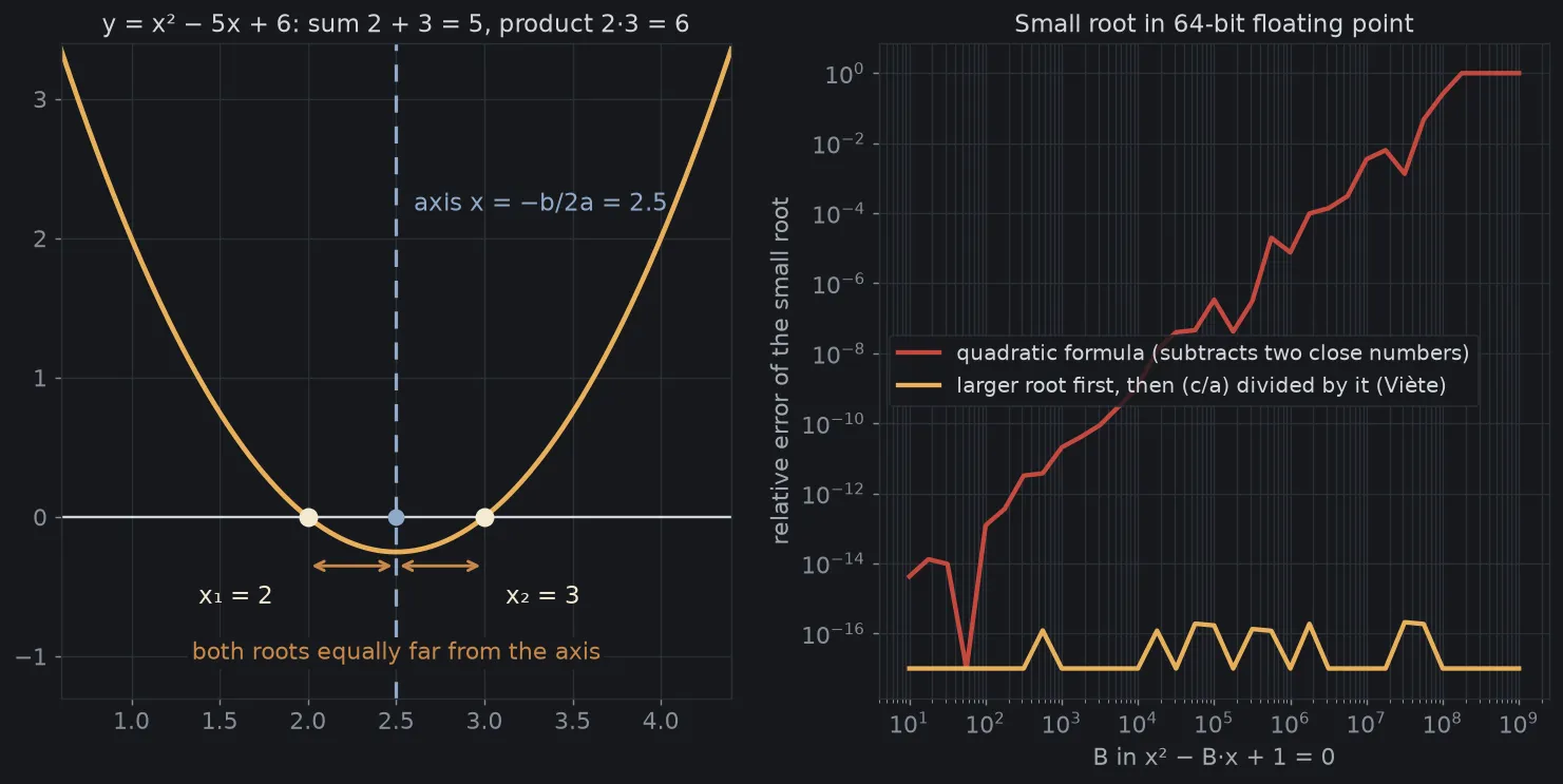
The first two lines confirm the theorem on the example from the start. The third line is the ball: the sum of the two times equals the flight time exactly. The next three lines are the gun (figure 3): the sum of the two roots of is 2.551 and their product is 1.000, so the angles 64.2° and 25.8° add up to exactly 90°, and both land at 800 meters. The maximum range is meters, at 45 degrees. The two lines about the gate (figure 2) give a sum of the feet of 0, a product of −36 and a width of 12 meters, and a 4-meter truck fits only within 4.47 meters of the centre line. The last two lines are about the computer: at the quadratic formula is off by more than a quarter of the true value, at it gives 0, while the product relation stays correct to the last digit. The red curve in figure 5 shows the error growing steadily as grows, not at a single bad point. This result is my own, with the standard 64-bit floats of Python; the 25.5% and the 0 depend on how the computer rounds, but the trend does not. The numbers about the gun and the gate are illustrative and ignore air resistance. You can change V, D or the coefficients of the gate to see how the angles and the width change.
Back to x² − 5x + 6
The folded sheet of paper at the start is the shortest picture of the theorem. The roots 2 and 3 land on each other when you fold along , and the grade 9 shortcut becomes something you can see: the sum of the roots is twice the position of the fold.
What the picture does not say is that the three coefficients of an equation hold more than we expect. They tell where the roots are, their sum and product, and the width of a gate. They tell when a ball and a shell are at a given height, and how to avoid a subtraction that destroys digits on a computer. Viète drew no parabola and used no computer, but letting a letter stand for a coefficient was the step that made all of these statements writable in one line.
Free geometry illustrations for students and teachers: EyeViz.
Tài liệu tham khảo
- [1]Vieta's formulas. Wikipedia.
- [2]François Viète. Wikipedia.
- [3]Quadratic equation. Wikipedia.
- [4]Parabola. Wikipedia.
- [5]Projectile motion. Wikipedia.
- [6]Eigenvalues and eigenvectors. Wikipedia.
- [7]La Géométrie. Wikipedia.
- [8]Thời điểm di dời cổng Parabol của Đại học Bách khoa Hà Nội (Vietnamese). VOV.VN (Voice of Vietnam), 2026.
- [9]Niccolò Fontana Tartaglia. Wikipedia.