What is the Fourier transform? The FFT in MP3, JPEG and 5G
What the Fourier transform is, how an 1807 idea about heat ended up in Shazam, MP3, JPEG, Wi-Fi and MRI, and why the FFT made it fast enough to use.
Mục lục
You are sitting in a café and the speakers play a song you half recognise but cannot name. You open Shazam, hold up your phone, and three seconds later the screen shows the title and the artist. Through the clatter of cups, the chatter and the traffic outside, the phone still “hears” the right recording. What makes that possible, and what also sits inside every MP3 file, every JPEG photo, every Wi-Fi signal and every hospital MRI scanner, is the Fourier transform.
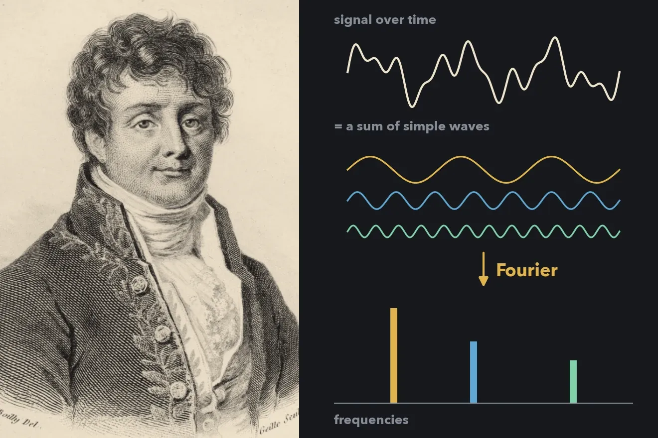
The short answer to “what is the Fourier transform”: it is a way to split a complicated signal into a sum of simple waves, and to say how fast each wave oscillates and how strong it is. A piece of music, a photo or a radio signal can all be rewritten this way. The FFT (fast Fourier transform) is the algorithm that lets a computer do that splitting so quickly that a phone can do it thousands of times a second.
This article has three legs. First, the man behind the name: an engineer who followed Napoleon to Egypt and was then told by the greatest mathematicians in France that his work lacked rigour. Next, the longest part: the places where Fourier works around you every day. Finally, the algorithm: how a computer calculates the Fourier transform, and why a “split in half” trick from 1965 is ranked among the most important algorithms of the 20th century.
What is the Fourier transform? Taste the broth, read the recipe
Picture a good cook tasting a spoonful of Vietnamese pho broth and saying: “Lots of cinnamon, a fair amount of star anise, a little charred ginger, a bit too much rock sugar.” The broth is one blended liquid; you cannot separate it by eye. But a well-trained tongue can read back the recipe: how much of each spice.
The Fourier transform does exactly that with signals. The input is the “broth”: a squiggly line recorded by a microphone, one number per instant. The output is the “recipe”: a list of frequencies, each with an amount.
Frequency is how many times a wave repeats each second, measured in hertz (Hz). A string vibrating 262 times a second gives the middle C of a piano. Faster, at 330 times, you hear an E. A higher note means a higher frequency, just as a fan sounds shriller the faster its blades spin.
When you press C, E and G together (a C major chord), the air does not vibrate as three separate waves. The three waves add up to a single line that looks messy, like the top half of Figure 1. Your ear still hears three notes, because your inner ear holds thousands of hair cells, each group sensitive to one band of frequencies, like a row of tiny tuning forks. The Fourier transform is the mathematical version of that inner ear: it looks at the squiggle and returns three clean lines at 262, 330 and 392 Hz, as in the bottom half of the figure.
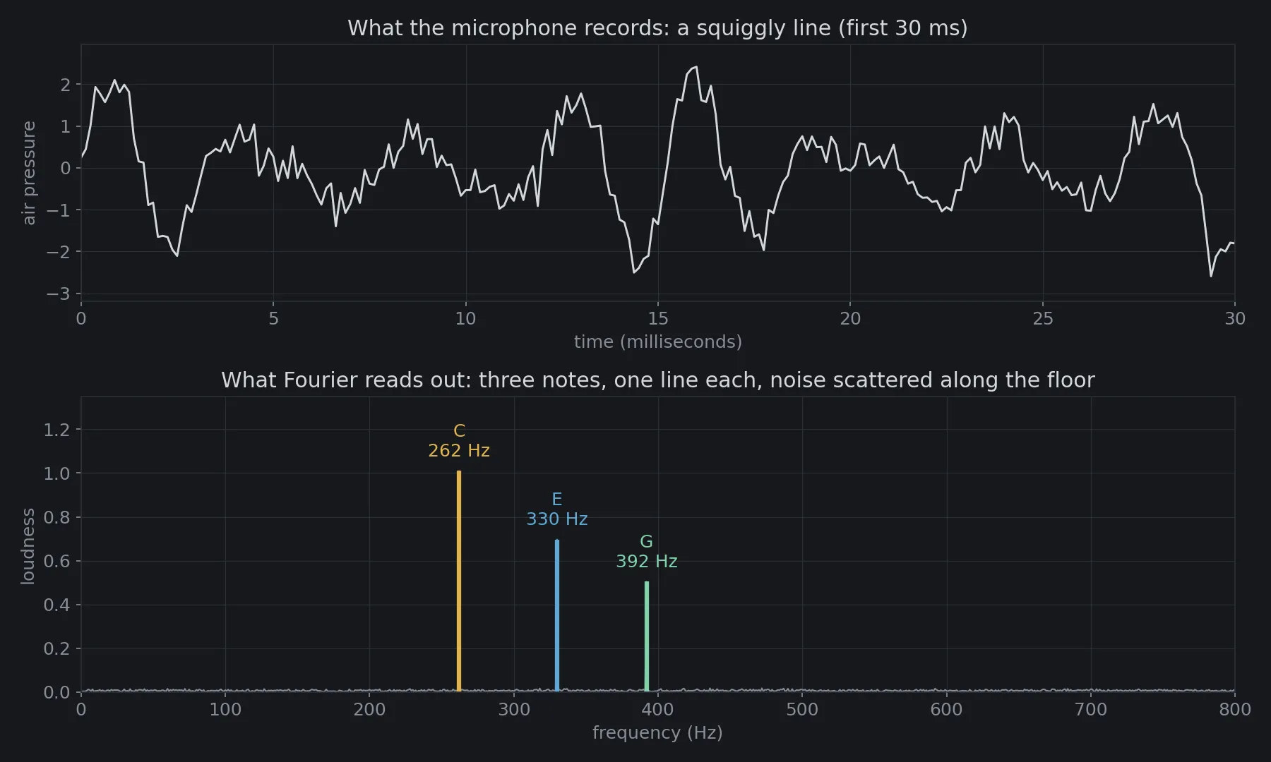
The key point is that this split is reversible. With the recipe in hand, you can cook the same broth again: add the waves back in the right amounts and you recover the original signal. So you can step over to the “frequency side” to work (remove, fix, compare) and then come back. Almost every application below follows the same rhythm: step over to the frequency side, do something that is much easier there, then come back.
The teacher who studied heat
Jean-Baptiste Joseph Fourier was born on 21 March 1768 in Auxerre, in central France, the son of a tailor. His mother passed away when he was nine, and his father the following year. The orphaned boy was placed by monks in the town’s military school, excelled at mathematics, and later returned to teach at that same school [1].
The French Revolution pulled him into local politics. In July 1794, in the middle of the Terror, he was arrested and for a time feared the guillotine. Robespierre fell soon after, the political climate changed, and Fourier was released [1]. He went to Paris and taught at the newly founded École Polytechnique.
In 1798 Napoleon invaded Egypt and took more than a hundred scholars with him. Fourier was one of them, serving as secretary of the Institute of Egypt in Cairo and collating the expedition’s scientific and archaeological findings. Back in France in 1801, he was appointed by Napoleon as prefect of the Isère department, based in Grenoble. By day he drained marshes and built a road towards Turin. In the evenings he studied a question that seems almost mundane: how does heat spread through a metal bar?
Imagine heating a few spots on an iron bar, hot here and cool there in a jagged pattern, then taking it off the fire. A few minutes later the hot spots have blurred into each other, the temperature along the bar has become smooth, and then the whole bar cools evenly. Fourier saw the easiest way to describe this: write the initial temperature profile as a sum of sine curves. Each sine curve cools in its own very simple way: it keeps its shape and just gets lower. The more tightly it wiggles (the higher its frequency), the faster it fades. That is why the jagged hot spots disappear first, leaving only a gentle arch. A hard problem (an arbitrary shape changing over time) becomes many easy problems (each sine wave shrinking), added together.
On 21 December 1807 he presented his memoir On the Propagation of Heat in Solid Bodies to the Paris Institute. It contained a bold claim: any function, even one with sharp corners or jumps, can be written as a sum of sine waves. Lagrange and Laplace, the two biggest names in French mathematics at the time, objected [1]. To them, sine waves were perfectly smooth. How could adding smooth, rounded things ever produce a vertical wall?
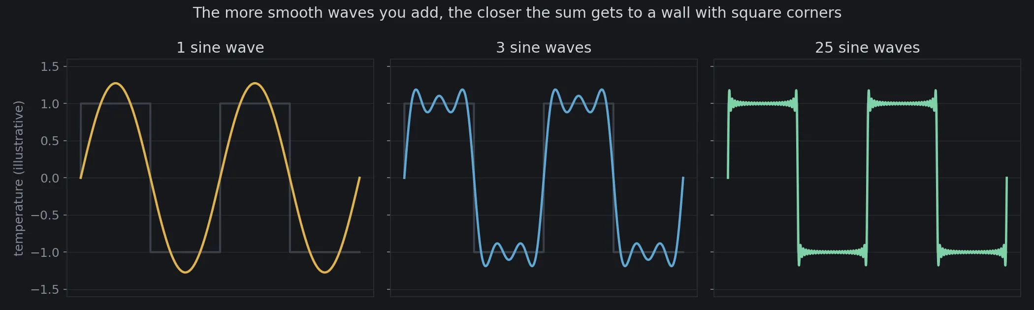
Figure 2 shows the answer. One sine wave is far from a square wave. Three already look like steps. Twenty-five are almost vertical. Add infinitely many and the sum approaches the square wave, even though every single wave is smooth. Just as enough small bricks can build a wall with a perfect right angle.
In 1811 the Institute chose heat propagation as the subject of its grand prize. Fourier entered and won, but the committee’s report said that the way he arrived at his equations “is not exempt of difficulties” and that his analysis “still leaves something to be desired on the score of generality and even rigour” [1]. Because of those reservations, the work was not printed. Only in 1822 did it appear as The Analytical Theory of Heat (Théorie analytique de la chaleur) [2], the same year he became permanent secretary of the Academy of Sciences. In 1824 he also wrote about the temperature of the Earth, a paper many historians regard as one of the earliest descriptions of what we now call the greenhouse effect [3].
Fourier passed away in Paris on 16 May 1830. A few weeks earlier, a prize entry from an 18-year-old named Évariste Galois had been sent to him. That manuscript was lost with him. His “insufficiently rigorous” claim of 1807, meanwhile, was later made rigorous by Dirichlet, Riemann and generations after them, and grew into a major branch of mathematics: Fourier analysis.
Where is the Fourier transform in your phone?
Two centuries later, Fourier spends most of his time working not with heat but with sound, images and radio waves. Here are six places you touch it every day, each following the same rhythm of “step over to the frequency side, do one thing, come back”.
Shazam: recognising a song by its constellation
Shazam does not compare sound waves with its music library. Two recordings of the same song, a clean studio version and one captured through café speakers, have completely different waveforms. What stays the same is which notes ring out strongly, and when.
So the app cuts the recording into very short frames, each a small fraction of a second, and computes a Fourier transform for each frame. Lining the results up over time gives a spectrogram: time on the horizontal axis, frequency on the vertical axis, brightness for strength. A spectrogram is like printed sheet music: one look tells you which note sounds when.
According to the 2003 paper by Avery Wang, who designed Shazam’s algorithm, the system keeps only the most prominent peaks of the spectrogram, the points much louder than their surroundings [4]. The rest, including most of the noise, is discarded. What is left looks like a starry sky, and Wang called it a “constellation map”. Each pair of nearby stars is encoded as a small “fingerprint”: the frequency of the first star, the frequency of the second, and the time between them.
When you press the button, the few seconds you recorded are turned into a batch of such fingerprints and looked up in a fingerprint index of millions of songs. The song with the most matching fingerprints, in the right time order, is the answer. Café noise may hide many stars, but enough of the remaining ones lining up in the right rhythm is enough, just as you can recognise the Big Dipper even when clouds cover part of the sky.
MP3 and AAC: throwing away what your ear cannot hear
One minute of CD audio takes about 10 MB: 44,100 samples per second, two channels, 16 bits per sample, or about 1,411 kilobits per second. A common MP3 runs at 128 kilobits per second, about 11 times smaller, and most listeners struggle to tell the difference. Where did the missing data go?
The answer lies in how human hearing works. If you talk next to someone drilling into a wall, your voice is drowned out: it is still there, but your brain does not hear it. This is called masking. A loud sound at one frequency makes quieter sounds at nearby frequencies “invisible”.
An MP3 encoder [5] cuts the music into short frames and moves them to the frequency side. A psychoacoustic model, itself built on Fourier analysis, estimates which frequencies are masking which in that frame. The masked or very quiet components are stored very coarsely or dropped, and the bits go to what the ear actually hears. At the other end, the player runs the inverse transform to rebuild the sound. This is lossy compression: you cannot get the original back, but what is lost is what you could not hear anyway.
JPEG: pictures are waves too
It sounds odd, but a picture also has “frequencies”. A patch of blue sky, where brightness changes very slowly from place to place, is a low-frequency region. Strands of hair, letters, the edges of leaves, where brightness changes abruptly within a few pixels, are high-frequency regions. The two-dimensional Fourier transform splits an image into a sum of light-and-dark “stripe patterns” of different widths, like pieces of striped fabric, some with wide stripes and some with fine ones, layered in every direction.
The human eye is far more sensitive to large patches than to fine detail. That is the opportunity for compression. Figure 3 runs a crude experiment: take the Fourier transform of Fourier’s portrait, keep only a small share of the strongest frequencies, throw away the rest, and transform back.
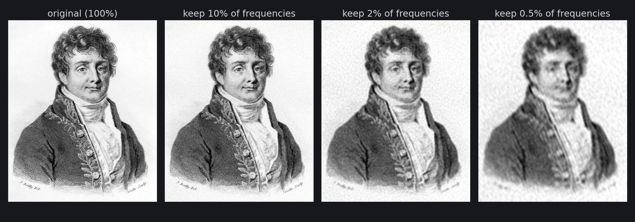
With only 10% of the numbers, the image barely changes. At 2%, the face is still clearly recognisable. The 1992 JPEG standard [6] does this more cleverly. It splits the image into 8×8-pixel blocks and turns each block into 64 numbers with the discrete cosine transform (DCT, a close relative of the Fourier transform, published in 1974 [7]). The first number is the block’s average brightness; the following ones are stripe patterns that get finer and finer. The numbers for the fine stripes are rounded aggressively, most of them to 0. The “quality” slider when you save an image is exactly this level of rounding. Push it too low and you will see the image break into small squares: those are the 8×8 blocks showing through.
Next time WhatsApp or Facebook compresses a photo you send, remember that the first thing to go is the finest stripe patterns, the details your eye notices least.
Wi-Fi, 4G, 5G: splitting one road into a thousand lanes
To send lots of data over radio, the naive approach is to change the signal very quickly on one frequency. The trouble is that radio waves bounce off walls, buildings and cars, so they reach the receiver along many paths of different lengths. The delayed copies pile up like echoes in a cave. When the signal changes too fast, one bit lands on top of the next and nobody can read it.
The solution used by Wi-Fi, 4G and 5G alike is called OFDM (orthogonal frequency-division multiplexing). Instead of one lane with extremely fast traffic, it divides the band into hundreds or thousands of narrow lanes, called subcarriers, each carrying a share of the data at a slow pace. Because each lane is slow, the echoes do almost no harm. It is like replacing one person sprinting down the street with flyers by a thousand people, each standing at one door and handing them out calmly.
The hard part is creating and separating thousands of waves at once, and that is Fourier’s job. The transmitter places the data into “frequency slots” and runs an inverse Fourier transform to produce a single signal that goes out over the air. The receiver takes that signal and runs a Fourier transform to separate the thousands of lanes and read each one. In 4G LTE with 20 MHz of bandwidth there are 1,200 subcarriers 15 kHz apart, using an FFT of size 2,048 [8], and the phone runs that operation tens of thousands of times every second. Without a fast FFT, the phone in your pocket could not receive 4G.
MRI scanners: imaging by frequency
A hospital MRI scanner does not take pictures the way a camera does. It places the body in a very strong magnetic field, excites the hydrogen nuclei in water and fat, and listens to the radio signals they emit. By varying the magnetic field with position, the machine makes each spot in the body “sing” at a slightly different frequency.
What the machine records is therefore not an image but the frequency side of the image, which engineers call “k-space”. An inverse Fourier transform in two (or three) dimensions turns that data into the slice of brain or knee that the doctor reads. Richard Ernst received the 1991 Nobel Prize in Chemistry precisely for developing Fourier-transform nuclear magnetic resonance, the foundation of how today’s MRI scanners acquire their signals [9].
Voice assistants and AI that “listens”
When you talk to a voice assistant or use speech-to-text, the AI model usually does not take the raw sound wave. It takes a spectrogram, much like Shazam’s. For example, OpenAI’s Whisper speech recognition model cuts audio into 25-millisecond frames, sliding forward every 10 milliseconds, and feeds the model 80 frequency bands per frame [10]. To the AI, your voice is a frequency “image”, and many techniques built for images are reused on it.
The smaller applications are too many to list: the bass and treble controls on your phone, noise filters in calls, seismometers telling earthquakes from explosions, the oscilloscopes of electrical engineers, multiplying two numbers with millions of digits. That last one returns in the algorithm section.
How does a computer calculate the Fourier transform?
We have seen what the Fourier transform does. The rest answers a programmer’s question: how do you calculate it, and how much work does it take?
Step 1: turn sound into a list of numbers
A computer cannot store a continuous line. It samples: it measures the signal at regular intervals, for example 44,100 times a second for CD audio, giving a list of numbers . It is like filming a runner: a film is just a sequence of still frames, but if they are dense enough you still see motion.
How dense is dense enough? The Nyquist–Shannon sampling theorem says you must sample faster than twice the highest frequency in the signal. Human hearing reaches about 20,000 Hz, so CDs use 44,100 samples per second, a little more than double. Sample more sparsely and high frequencies “disguise” themselves as low ones. You have seen this in films: a car’s wheels speeding along look as if they are turning slowly, or even backwards, because the camera does not capture frames fast enough.
Step 2: try every test wave
The discrete Fourier transform (DFT) asks one question for each frequency: how much does this signal “resemble” a wave of frequency ? Measuring resemblance is simple: multiply each sample of the signal by the matching sample of the test wave, then add everything up. If the signal contains that wave, the products share the same sign and pile up into a large number. If not, positive and negative products cancel out and the sum is close to 0.
Think of pushing a child on a swing. Push in time with the swing and every push adds up, sending it higher. Push out of time and one push cancels the next, and the swing barely moves. The DFT “pushes” the signal at each rhythm and sees which rhythms make it “fly”.
As a formula:
The factor looks scary, but it is just a point running around a circle: as increases it turns steadily around the unit circle, times in steps, like a second hand going round times in a minute. Using a point on a circle instead of a single sine wave lets one complex number capture both the loudness and the phase (whether the wave starts early or late). The size gives the height of each line in Figure 1.
The cost: for each of the frequencies, we add up products. That is about multiplications in total. One second of CD audio has 44,100 samples, so nearly 2 billion multiplications for a single transform. A signal of a million samples needs about a trillion multiplications. In 1960 that was impossible. Even today, a phone that must run tens of thousands of transforms a second for 4G could never afford .
The FFT: divide and conquer
The most widely used FFT, the Cooley–Tukey algorithm, rests on one observation: split the list into even and odd positions.
Separate the samples into two groups: those at even positions and those at odd positions . Each group has samples. Let be the DFT of the even group and the DFT of the odd group. Rearranging the DFT formula a little (all you need is ) gives:
Those two lines are the whole secret. Each pair , is used twice: once for and once for , differing only by a plus or minus sign. It is like cooking one pot of broth and splitting it between two dishes, beef pho and chicken pho, instead of cooking two pots. Engineers call this criss-cross pair of operations a “butterfly”, because drawn out it looks like a pair of wings.
Then we do the same to and themselves: each group of splits into two groups of , and so on until each group holds a single sample. The DFT of one sample is the sample itself, nothing to compute. This is the same divide and conquer you met in binary search and in the recursive solution of the Tower of Hanoi: split a problem into smaller problems of the same kind, then combine their answers.
Each level of splitting costs about operations to combine the butterflies. The number of levels is the number of times you halve to reach 1, which is . For a million samples that is only about 20 levels, since , just as folding a sheet of paper in half 20 times gives a million layers. The total work is about instead of .
| Samples | Direct DFT () | FFT () | Speed-up |
|---|---|---|---|
| 1,024 | 1.05 million | 10,240 | 102 × |
| 65,536 | 4.3 billion | 1.05 million | 4,096 × |
| 1,048,576 | 1.1 trillion | 21 million | 52,429 × |
If each operation takes a billionth of a second, the last row means about 18 minutes versus 0.02 seconds. That gap decides which technologies can exist. An MRI scanner that needs hours to rebuild each slice, or a phone that needs 18 minutes for every millisecond of 4G signal, would be useless to everyone.
The halving trick needs to be a power of 2 (1,024, 2,048, 4,096…), which is why those numbers appear all over telecommunications. Other FFT variants handle any , but the core idea is still to split up and reuse.
The idea of “reuse” reaches beyond signal processing. Multiplying two huge numbers, each with millions of digits, can be turned into multiplying two polynomials, and the fastest way to multiply polynomials is to go to the frequency side with an FFT, multiply pair by pair, and come back. The libraries that compute to trillions of digits all rely on this trick.
Gauss had it 160 years earlier, then the Cold War found it again
The history of the FFT has a memorable twist. Around 1805, Carl Friedrich Gauss, who a few years earlier had found the lost asteroid Ceres again, needed to interpolate the orbits of two other asteroids, Pallas and Juno, from discrete measurements. To calculate quickly by hand, he came up with exactly the splitting trick we just saw, including its recursive use [12]. But he did not publish it. The manuscript, written in Latin, was printed only after he passed away, in his collected works of 1866, and went almost unnoticed [13]. Remarkably, Gauss did this even before Fourier presented his memoir on heat in 1807.
A hundred and sixty years later, in the early 1960s, the United States and the Soviet Union were negotiating a ban on nuclear weapons tests. To sign such a treaty, the US needed a way to check whether the Soviets were keeping their word without entering their territory. The most practical way was to place seismometers in neighbouring countries and analyse ground vibrations: an underground explosion has a different “frequency signature” from an earthquake. But with dozens of stations and hours of data, the DFT was far too slow.
According to accounts of the algorithm’s history, John Tukey, a statistician at Princeton University, conceived the idea during a meeting of President Kennedy’s Science Advisory Committee about this very problem [13]. Richard Garwin, an IBM physicist also present, saw its potential at once and put Tukey in touch with James Cooley, a mathematician at IBM’s research lab. Garwin did not tell Cooley the real purpose. Cooley was told the algorithm was needed to find periodicities in a crystal of helium-3.
In 1965 Cooley and Tukey published a five-page paper, “An Algorithm for the Machine Calculation of Complex Fourier Series” [11]. Analog-to-digital converters were becoming cheap and fast at just that moment, and the FFT spread extremely quickly. In 1994 the MIT mathematician Gilbert Strang called the FFT “the most important numerical algorithm of our lifetime” [15]. In 2000 the journal Computing in Science & Engineering put it on its list of the ten most influential algorithms of the 20th century [14]. Only several years after the 1965 paper did anyone realise that Gauss had had the idea at the start of the 19th century.
Split a chord yourself
The code below produces exactly Figure 1. It builds one second of a C major chord from three sine waves (frequencies rounded to the nearest hertz), adds random noise with the fixed seed 1768, the year Fourier was born, and uses the FFT to read the three notes back. The last part compares the speed of a DFT computed straight from its definition (multiplying by an matrix) with numpy’s FFT on 2,048 samples. You only need numpy and matplotlib.
import time
import matplotlib.pyplot as pltimport numpy as np
plt.rcParams.update({"figure.facecolor": "#16181c", "axes.facecolor": "#16181c", "text.color": "#d4d7dc",                     "axes.edgecolor": "#2a2e35", "axes.labelcolor": "#878d97",                     "xtick.color": "#878d97", "ytick.color": "#878d97", "font.size": 12})
# 1. One second of a C major chord: C, E and G played together, plus a little noisefs = 8_000                                   # sampling rate: 8,000 samples per secondt = np.arange(fs) / fs                       # 1 secondNOTES = {"C": (262, 1.0), "E": (330, 0.7), "G": (392, 0.5)}   # frequency (Hz, rounded), loudnessrng = np.random.default_rng(1768)            # fixed seed: the year Fourier was bornx = sum(a * np.sin(2 * np.pi * f * t) for f, a in NOTES.values()) + 0.3 * rng.standard_normal(fs)
# 2. Fourier transform with the FFT: 8,000 numbers over time become 4,001 "amounts" over frequencyX = np.fft.rfft(x)freqs = np.fft.rfftfreq(len(x), 1 / fs)      # bins are 1 Hz apartamplitude = 2 * np.abs(X) / len(x)           # scale back to each wave's loudnessfor name, (f, a) in NOTES.items():    k = np.argmin(np.abs(freqs - f))    print(f"{name}: put in {a:.2f}, FFT reads {amplitude[k]:.2f} at {freqs[k]:.0f} Hz")
# 3. Speed: the DFT straight from its definition (N² multiplications) versus the FFT (N log N)N = 2_048n = np.arange(N)W = np.exp(-2j * np.pi * np.outer(n, n) / N)   # N × N matrix of "test waves"start = time.perf_counter(); X_slow = W @ x[:N]; t_slow = time.perf_counter() - startstart = time.perf_counter(); X_fast = np.fft.fft(x[:N]); t_fast = time.perf_counter() - startprint(f"N = {N}: both methods agree: {np.allclose(X_slow, X_fast)}")print(f"direct DFT: {t_slow * 1e3:.1f} ms · FFT: {t_fast * 1e3:.3f} ms")
# 4. Plot: top is what the microphone records, bottom is what Fourier reads outCOLOR = {"C": "#e0b44c", "E": "#5fa8d3", "G": "#7fd1a8"}fig, (a1, a2) = plt.subplots(2, 1, figsize=(12, 7.2), gridspec_kw={"height_ratios": [1, 1.15]})ms = t * 1000a1.plot(ms, x, color="#d4d7dc", lw=1.4)a1.set(xlim=(0, 30), xlabel="time (milliseconds)", ylabel="air pressure",       title="What the microphone records: a squiggly line (first 30 ms)")a2.plot(freqs, amplitude, color="#878d97", lw=1)for name, (f, a) in NOTES.items():    k = np.argmin(np.abs(freqs - f))    a2.vlines(freqs[k], 0, amplitude[k], color=COLOR[name], lw=3)    a2.text(freqs[k], amplitude[k] + 0.05, f"{name}\n{f:.0f} Hz", color=COLOR[name], ha="center", va="bottom")a2.set(xlim=(0, 800), ylim=(0, 1.35), xlabel="frequency (Hz)", ylabel="loudness",       title="What Fourier reads out: three notes, one line each, noise scattered along the floor")for a in (a1, a2):    a.grid(color="#2a2e35", lw=0.6)    a.set_axisbelow(True)fig.tight_layout()fig.savefig("hop-am-fourier-en.png", dpi=150)
Output:
C: put in 1.00, FFT reads 1.01 at 262 HzE: put in 0.70, FFT reads 0.70 at 330 HzG: put in 0.50, FFT reads 0.50 at 392 HzN = 2048: both methods agree: Truedirect DFT: 12.6 ms · FFT: 0.115 msEven though each sample carries noise of about 0.3 units, the FFT reads back each note’s loudness almost exactly, because random noise is spread evenly over 4,001 frequency bins while each note is concentrated in one. This is also why Shazam can still recognise a song in a noisy café. The timings were measured on the author’s machine; yours will differ, but the FFT is still tens to hundreds of times faster at , and the gap widens as grows. Try changing a frequency in NOTES to an off-grid value such as 261.63 Hz and watch its line “leak” into the neighbouring bins: one second of signal can only tell apart frequencies 1 Hz apart.
From a hot iron bar to your phone
In 1807 Fourier only wanted to know how an iron bar cools. To answer, he made a claim that the best minds of his day considered insufficiently rigorous: every shape is a sum of simple waves. In 1805 Gauss had found a fast way to compute it but left it in a drawer. In 1965, worries about underground nuclear explosions led two scientists to find that method again.
Today, every time you play a song, send a photo, pick up a 4G signal or get an MRI scan, the idea of the orphaned teacher from Auxerre runs thousands of times in a few seconds. Next time Shazam names a song after three seconds, you will know that in those three seconds your phone tasted the “broth” of sound and read out its recipe.
If you enjoy “one algorithmic idea behind something you use every day”, read on about Bloom filters or image search.
Free geometry illustrations for students and teachers: EyeViz.
Tài liệu tham khảo
- [1]J. J. O'Connor and E. F. Robertson. Joseph Fourier, biography. MacTutor History of Mathematics, University of St Andrews.
- [2]Joseph Fourier. Théorie analytique de la chaleur. Firmin Didot, Paris, 1822.
- [3]Joseph Fourier. Remarques générales sur les températures du globe terrestre et des espaces planétaires. Annales de Chimie et de Physique, 27, 136–167, 1824.
- [4]Avery Li-Chun Wang. An Industrial-Strength Audio Search Algorithm. Proceedings of ISMIR 2003, 2003.
- [5]ISO/IEC 11172-3: Coding of moving pictures and associated audio, Part 3: Audio (MPEG-1 Audio, including Layer III/MP3). ISO/IEC, 1993.
- [6]ITU-T T.81: Digital compression and coding of continuous-tone still images (JPEG). ITU-T, 1992.
- [7]N. Ahmed, T. Natarajan and K. R. Rao. Discrete Cosine Transform. IEEE Transactions on Computers, C-23(1), 90–93, 1974.
- [8]3GPP TS 36.211: Evolved Universal Terrestrial Radio Access (E-UTRA); Physical channels and modulation. 3GPP.
- [9]The Nobel Prize in Chemistry 1991: Richard R. Ernst. NobelPrize.org.
- [10]A. Radford, J. W. Kim, T. Xu, G. Brockman, C. McLeavey and I. Sutskever. Robust Speech Recognition via Large-Scale Weak Supervision (Whisper). arXiv:2212.04356, 2022.
- [11]J. W. Cooley and J. W. Tukey. An Algorithm for the Machine Calculation of Complex Fourier Series. Mathematics of Computation, 19(90), 297–301, 1965.
- [12]M. T. Heideman, D. H. Johnson and C. S. Burrus. Gauss and the History of the Fast Fourier Transform. IEEE ASSP Magazine, 1(4), 14–21, 1984.
- [13]Cooley–Tukey FFT algorithm. Wikipedia.
- [14]J. Dongarra and F. Sullivan. Guest Editors’ Introduction: The Top 10 Algorithms. Computing in Science & Engineering, 2(1), 22–23, 2000.
- [15]Gilbert Strang. Wavelets. American Scientist, 82(3), 250–255, 1994.