Tower of Hanoi: dynamic programming explained simply
The 64-disc Tower of Hanoi takes 585 billion years; one extra peg cuts it to 5 hours. That is dynamic programming, now in routers, phones and DNA.
Mục lục
There is a puzzle named after the capital of Vietnam that almost every computer science student in the world meets at least once: the Tower of Hanoi. Three pegs, a stack of discs from large at the bottom to small at the top, and a task that sounds simple: move the whole stack to another peg.
With 64 discs, if you move one disc per second and never make a mistake, you need about 585 billion years, more than 40 times the age of the universe. Add just a fourth peg, and the figure drops to about 5 hours. Finding that 5-hour strategy takes one of the most useful ideas in computer science: dynamic programming.
Dynamic programming fits in one sentence: split a big problem into subproblems, solve each subproblem exactly once, write the answer in a table, and reuse it. The same idea is at work when your phone decodes a noisy radio signal, when your keyboard suggests a spelling fix, when biologists compare two stretches of DNA, and when Internet routers pick a path for your data.
The first half of this article needs no programming. The second half has the formulas and a short piece of code so you can check every number yourself.
What is the Tower of Hanoi?
The rules are just three:
- There are three pegs. At the start every disc sits on the left peg, largest at the bottom, getting smaller toward the top.
- Each move lifts the top disc of one peg and puts it on another peg.
- A larger disc may never sit on a smaller one.
The goal is to move the whole stack to the right peg.
The game was first sold in Paris in 1883 as La Tour d’Hanoï. The inventor signed as “Professor N. Claus de Siam”, a pen name: it is an anagram of “Lucas d’Amiens”. The real author was Édouard Lucas, a French mathematician known for the Lucas numbers and for proving that is prime, which stayed the largest known prime for the next 75 years[1][2].
Lucas never explained why he picked Hà Nội. In the early 1880s France was conquering northern Vietnam (French troops took the citadel of Hà Nội in 1882), so many people believe he chose an Eastern name that filled French newspapers at the time to give the toy an air of mystery.
The game came with a legend (most likely spun by Lucas himself as advertising, not a real old tale): in a temple in India, priests move 64 golden discs day and night by exactly these rules. When they finish, the world will end. We will soon see why there is no need to worry.
Solving the Tower of Hanoi: one single idea
Try 3 discs, named 1, 2, 3 from small to large. You can find a 7-move solution by trial and error. But the way of thinking matters more than the solution.
Look at the largest disc. To lift it, every other disc must have left the left peg. To put it on the right peg, the right peg must be empty. So at the moment the largest disc moves, all the other discs must be sitting together on the middle peg. There is no other way.
The solution follows by itself, in three stages:
- Move the top discs from the left peg to the middle peg (using the right peg as a stopover).
- Move the largest disc to the right peg. One move.
- Move the discs from the middle peg to the right peg, on top of the largest disc.
Stages 1 and 3 are the very same game with one disc fewer. And the disc game is solved by the same three stages with discs, and so on until only one disc is left, which takes a single move. Solving a problem through a smaller version of itself is called recursion.
Let be the minimum number of moves for discs. The three stages give:
Step by step: , , , , … Each extra disc doubles the moves and adds one. The pattern is .
Because the argument “the largest disc must travel alone between two clean-ups” leaves no way out, is not just one way to play but the fewest moves possible, and the optimal solution is unique.
Back to the temple. With 64 discs:
At one move per second the priests need about years, that is 585 billion years. The universe is 13.8 billion years old. The world is quite safe.
One more peg changes everything
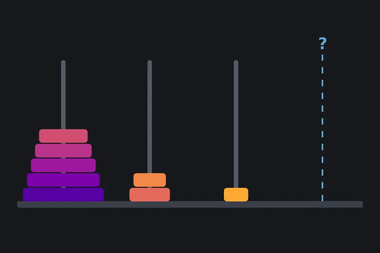
In 1907 the English puzzle maker Henry Dudeney put a variant in his book The Canterbury Puzzles: an innkeeper must move 8 cheeses of different sizes across 4 stools, again never placing a larger cheese on a smaller one[3]. This is now called Reve’s puzzle, or the four-peg Tower of Hanoi.
With one more empty peg, we are no longer forced to pile every disc into one place. The most natural strategy, published by J. S. Frame and B. M. Stewart in 1941, goes like this[4]:
- Take the smallest discs from the top and move them to a spare peg to “park” there, using all 4 pegs.
- Move the remaining large discs to the target peg. One peg is now taken by the pile of small discs (large discs may not sit on them), so only 3 pegs are usable: moves.
- Move the small discs from their parking spot onto the target peg, again with all 4 pegs.
Let be the number of moves with 4 pegs. For a fixed , the total is . But which ? Park too few discs and the 3-peg middle stage is ruinously expensive; park too many and the parking itself costs a lot. There is no reason to guess in advance; the safe way is to try every and pick the cheapest:
This formula has one special feature: to compute you need for every smaller . This is exactly where dynamic programming comes in.
What is dynamic programming?
Try computing the “straightforward” way: write a function that tries each , and for each calls itself to compute .
The trouble is that the subproblems overlap. Computing needs . Computing again needs . Computing again needs … The question “what is ?” gets asked hundreds of times, and each time the machine dutifully works it out from scratch as if it had never seen it. The number of function calls is exactly : over 2 million for 22 discs, and for 64 discs. This “straightforward” approach is almost as slow as the temple.
The dynamic programming way: fill a table from small to large.
| 1 | 2 | 3 | 4 | 5 | 6 | 7 | 8 | 9 | 10 | |
|---|---|---|---|---|---|---|---|---|---|---|
| 3 pegs: | 1 | 3 | 7 | 15 | 31 | 63 | 127 | 255 | 511 | 1023 |
| 4 pegs: | 1 | 3 | 5 | 9 | 13 | 17 | 25 | 33 | 41 | 49 |
| best | 1 | 1 | 1 | 2 | 3 | 3 | 4 | 5 | 6 |
To fill the cell , you only look at the 9 cells already filled to its left, try 9 values of , and keep the smallest. Every cell is computed once. All the way up to 64 discs that is only trials, done by a computer in under a millisecond.
Look at the column : 33 moves. That is exactly the answer to Dudeney’s 8-cheese puzzle from 1907.
And for 64 discs: moves. At one move per second, about 5 hours 7 minutes. One extra peg has turned 585 billion years into an afternoon.
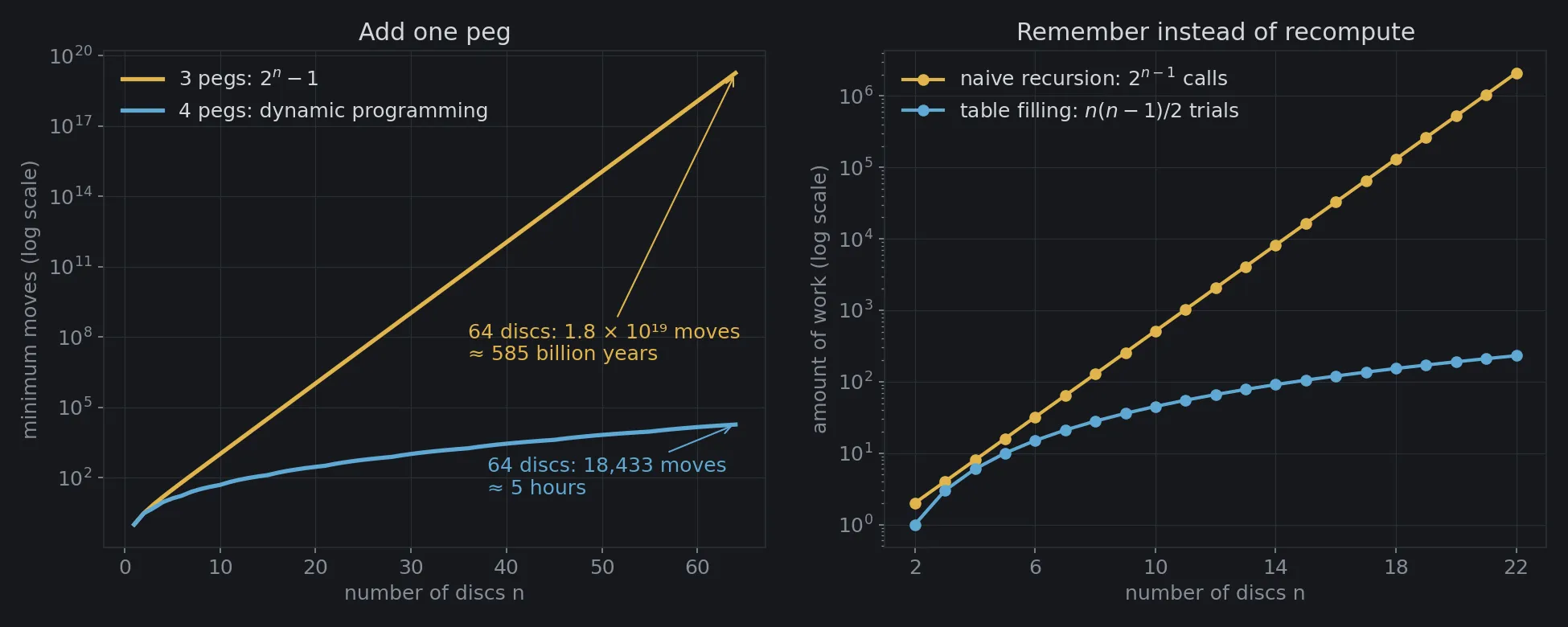
Figure 1 shows two exponential explosions being defused. On the left, in the game itself: with one more peg, the number of moves grows far more slowly than an exponential. On the right, in the way we compute: by remembering old results, the work drops from exponential to merely quadratic.
Two conditions for dynamic programming
Not every problem can be “solved by filling a table”. Two conditions must hold:
- Optimal substructure: the best solution of the big problem is built from the best solutions of the small ones. The best way to park the small discs inside the best -disc solution is itself the best -disc solution.
- Overlapping subproblems: the same small problem is asked many times. That is why remembering pays off. If the subproblems never repeat (as when you split a list in half to sort it), remembering helps nothing and plain recursion is enough.
The three-peg Tower of Hanoi offers only one choice at each step, so recursion is enough. The four-peg version forces us to choose among many values of , and every choice leads back to subproblems we have already met. That is the signature of a dynamic programming problem: you have to choose, and the choices lead back to the same small set of subproblems.
Why is it called “dynamic programming”?
The name seems to have nothing to do with tables or memory, and that was deliberate. It was coined by the American mathematician Richard Bellman while working at the RAND Corporation in the early 1950s. As he told it in his autobiography, RAND was funded by the US Air Force, and the Secretary of Defense at the time, Charles Wilson, had a pathological fear of the word “research”, let alone “mathematical research”. Bellman needed a name that no congressman could object to[6].
He picked programming, in the sense of the time, “planning and scheduling”, not writing code. He added dynamic because his problems unfolded over time, with decisions following one another, and because, in his words, “it’s impossible to use the word dynamic in a pejorative sense”.
Behind that somewhat political name lies a very compact rule Bellman called the principle of optimality: an optimal plan has the property that whatever step you are at, the rest of the plan must also be optimal from where you now stand. In road-trip terms: if the fastest route from Hà Nội to Hồ Chí Minh City passes through Đà Nẵng, then its stretch from Đà Nẵng to Hồ Chí Minh City must also be the fastest route between those two cities. Otherwise you could simply swap that stretch for a faster one.
Where is dynamic programming running around you?
Routing packets on the Internet
In 1958 Bellman applied exactly this principle to finding shortest paths[7]. Instead of trying every route, each point only needs to know “how far am I from the destination?”, and it works that out from its neighbours’ answers. My shortest distance equals the smallest value of (distance to a neighbour + that neighbour’s shortest distance). It is a table filled in step by step.
This algorithm, now called Bellman–Ford, underlies RIP, one of the earliest ways routers on the Internet exchanged routing tables[8]. Each router talks only to its neighbours, yet the whole network gradually learns the shortest path to everywhere.
Spell-checkers and file comparison
You type “dynamic programmign” and the computer suggests “programming”. To do that it must measure how different two words are: the fewest single-letter insertions, deletions or substitutions that turn one into the other. This quantity is called the edit distance (or Levenshtein distance).
Trying every possible edit is hopeless. Dynamic programming does this: build a table whose cell in row , column holds the distance between the first letters of the first word and the first letters of the second. Each cell only needs its three neighbours (left, above, upper-left diagonal) and picks the cheapest of three operations. The bottom-right cell is the answer[9]. Tools that compare two versions of a text or of source code (such as the diff command) solve a sister problem: finding the longest common part of two texts, so they can highlight the lines that were added and removed.
Comparing two stretches of DNA
Replace letters with the bases A, C, G, T and you have a basic tool of molecular biology. In 1970 Saul Needleman and Christian Wunsch published an algorithm that aligns two protein sequences with exactly that kind of table[10]. Whenever scientists ask “which mouse gene does this human gene resemble?”, or compare a new virus sample with known strains, their idea (along with its many variants and faster versions) is at work.
Your phone decoding a signal
Radio waves reaching your phone are always noisy. To correct errors, the sender encodes the data so that each bit depends on a few bits before it. The receiver must guess: which original bit sequence most likely produced this noisy signal? The number of possible sequences is enormous.
In 1967 Andrew Viterbi proposed a dynamic programming algorithm for this[11]: move forward in time, and at each moment keep only the best path leading to each state, discarding every worse one. The Viterbi algorithm is found in mobile networks, Wi‑Fi, satellite links and the classic generation of speech recognition systems. Viterbi later co-founded Qualcomm.
Shrinking a photo without squashing it
Want to make a landscape photo narrower without making the people in it look thinner? In 2007 Shai Avidan and Ariel Shamir proposed seam carving[12]: find a “seam” running from the top of the image to the bottom through the least important pixels (sky, water), then cut it out. The best seam is found with a table: the best cost to reach each pixel equals its own cost plus the cheapest of the three pixels directly above it. The idea lives on in the content-aware resizing features of photo editors.
Pricing options
In finance, the Cox–Ross–Rubinstein binomial tree (1979) prices an American option, one that can be exercised at any time before expiry, by working backward from the expiry date to today[13]. At every node of the tree, the holder compares “exercise now” with “hold on” (a value derived from the two nodes after it, already computed), and takes the larger. That is Bellman’s principle of optimality, applied to money.
When dynamic programming cannot save you
Dynamic programming turns exponential into polynomial when the number of distinct subproblems is small. The four-peg tower has only 64 subproblems: through . But in some problems the number of “states” to remember explodes on its own.
The travelling salesman problem (visit cities once each with the shortest total route) has a dynamic programming solution, but its table has about cells. With 30 cities that is over 30 billion cells and nearly a trillion operations. Bellman called this the curse of dimensionality: every extra dimension of the state multiplies the size of the table. That is why many real systems (map routing included) combine dynamic programming with estimation tricks, or switch to machine learning, where a neural network learns to “guess” the value of a cell instead of computing every cell exactly.
One distinction is worth keeping: the extra peg makes the game shorter; dynamic programming makes finding the strategy faster. They are different things. Dynamic programming does not remove a single move from the 3-peg game, because is already optimal. It only lets us find the best 4-peg strategy without trials.
Computing the four-peg tower yourself
The code below produces exactly Figure 1 and prints the table above. It implements two ways of computing : naive recursion (counting the function calls) and dynamic programming (filling a table), checks that both agree up to 22 discs, then uses the table to go all the way to 64 discs. There is no randomness, so every run gives the same numbers. You only need matplotlib; the naive part takes a few seconds.
import matplotlib.pyplot as plt
plt.rcParams.update({"figure.facecolor": "#16181c", "axes.facecolor": "#16181c", "text.color": "#d4d7dc",                     "axes.edgecolor": "#2a2e35", "axes.labelcolor": "#878d97",                     "xtick.color": "#878d97", "ytick.color": "#878d97", "font.size": 12})GOLD, BLUE = "#e0b44c", "#5fa8d3"N = 64
# 1. Three pegs: park n−1 discs on the spare peg, move the largest, bring n−1 discs back.def three_pegs(n):    return 2**n - 1
# 2. Four pegs (Frame–Stewart): park the top k discs on one peg using all 4 pegs,#    move the other n−k discs using 3 pegs, then bring the k discs back. Try every k.count = {"naive": 0}
def four_pegs_naive(n):    """Plain recursion: every repeated subproblem is solved again from scratch."""    count["naive"] += 1    if n <= 1:        return n    return min(2 * four_pegs_naive(k) + three_pegs(n - k) for k in range(1, n))
def four_pegs_dp(n_max):    """Dynamic programming: fill the table F[0..n_max] from small to large, each cell once."""    F, best_k, trials = [0, 1], [0, 0], 0    for n in range(2, n_max + 1):        candidates = {k: 2 * F[k] + three_pegs(n - k) for k in range(1, n)}        trials += len(candidates)        k = min(candidates, key=candidates.get)        F.append(candidates[k])        best_k.append(k)    return F, best_k, trials
F, best_k, trials = four_pegs_dp(N)print(" n | 3 pegs | 4 pegs | best k")for n in range(1, 11):    print(f"{n:2d} | {three_pegs(n):6d} | {F[n]:6d} | {best_k[n]}")print(f"n = 64: 3 pegs need {three_pegs(N):,} moves, 4 pegs only {F[N]:,}")years = three_pegs(N) / (365.25 * 24 * 3600)print(f"  one move per second: {years:.3e} years versus {F[N] / 3600:.1f} hours")
# 3. Count the naive calls (n from 2 to 22, to keep it quick) and compare with the table.n_count = list(range(2, 23))naive_calls = []for n in n_count:    count["naive"] = 0    assert four_pegs_naive(n) == F[n]    naive_calls.append(count["naive"])table_trials = [four_pegs_dp(n)[2] for n in n_count]print(f"n = 22: naive makes {naive_calls[-1]:,} calls, the table needs {table_trials[-1]} trials")print(f"n = 64: the table needs {trials} trials, naive would need 2^63 ≈ {2**63:.2e} calls")
fig, (a1, a2) = plt.subplots(1, 2, figsize=(13, 5.2))ns = range(1, N + 1)a1.semilogy(ns, [three_pegs(n) for n in ns], color=GOLD, lw=2.5, label="3 pegs: $2^n - 1$")a1.semilogy(ns, [F[n] for n in ns], color=BLUE, lw=2.5, label="4 pegs: dynamic programming")a1.annotate("64 discs: 1.8 × 10¹⁹ moves\n≈ 585 billion years", (N, three_pegs(N)), (36, 1e7),            color=GOLD, arrowprops=dict(arrowstyle="->", color=GOLD))a1.annotate("64 discs: 18,433 moves\n≈ 5 hours", (N, F[N]), (38, 2e1),            color=BLUE, arrowprops=dict(arrowstyle="->", color=BLUE))a1.set(xlabel="number of discs n", ylabel="minimum moves (log scale)", title="Add one peg")a1.legend(frameon=False, loc="upper left")
a2.semilogy(n_count, naive_calls, "o-", color=GOLD, lw=2, label="naive recursion: $2^{n-1}$ calls")a2.semilogy(n_count, table_trials, "o-", color=BLUE, lw=2, label="table filling: $n(n-1)/2$ trials")a2.set(xlabel="number of discs n", ylabel="amount of work (log scale)", title="Remember instead of recompute")a2.set_xticks(range(2, 23, 4))a2.legend(frameon=False, loc="upper left")for a in (a1, a2):    a.grid(color="#2a2e35", lw=0.6)fig.tight_layout()fig.savefig("thap-ha-noi-quy-hoach-dong-en.png", dpi=150)
The output:
n | 3 pegs | 4 pegs | best k 1 | 1 | 1 | 0 2 | 3 | 3 | 1 ...10 | 1023 | 49 | 6n = 64: 3 pegs need 18,446,744,073,709,551,615 moves, 4 pegs only 18,433 one move per second: 5.845e+11 years versus 5.1 hoursn = 22: naive makes 2,097,152 calls, the table needs 231 trialsn = 64: the table needs 2016 trials, naive would need 2^63 ≈ 9.22e+18 callsTo see the power of remembering with your own eyes, change range(2, 23) to range(2, 30): the naive part will run for minutes, while the table part still finishes instantly. Another way to add “memory” without building the table yourself is to put @functools.cache above four_pegs_naive; the number of times the function actually has to compute drops straight to the number of cells in the table.
Don’t solve again what you already know
The Tower of Hanoi is usually taught as a lesson in recursion, and rightly so. But the more interesting story lies in the fourth peg. When a problem forces you to choose, and each choice leads back to small questions you have met before, the smart move is to answer each small question exactly once and write it down.
It sounds almost too obvious, yet that obviousness helps routers pick paths, helps phones hear through noise, and helps biologists read DNA. Next time a problem seems to require trying billions of possibilities, ask: how many truly different small questions are hidden inside? If the answer is “not many”, you have just found a dynamic programming problem.
If you enjoy “one algorithmic idea behind something you use every day”, read on about binary search inside databases or Bloom filters.
Free geometry illustrations for students and teachers: EyeViz.
Tài liệu tham khảo
- [1]Andreas M. Hinz, Sandi Klavžar and Ciril Petr. The Tower of Hanoi – Myths and Maths (2nd ed.). Birkhäuser, 2018.
- [2]Tower of Hanoi. Wikipedia.
- [3]Henry Ernest Dudeney. The Canterbury Puzzles (The Reve's Puzzle), 1907.
- [4]J. S. Frame; B. M. Stewart. Solution to Advanced Problem 3918. The American Mathematical Monthly 48(3), 1941.
- [5]Thierry Bousch. La quatrième tour de Hanoï. Bulletin of the Belgian Mathematical Society – Simon Stevin 21(5), 2014.
- [6]Stuart Dreyfus. Richard Bellman on the Birth of Dynamic Programming. Operations Research 50(1), 2002.
- [7]Richard Bellman. On a Routing Problem. Quarterly of Applied Mathematics 16(1), 1958.
- [8]G. Malkin. RFC 2453: RIP Version 2. IETF, 1998.
- [9]Robert A. Wagner and Michael J. Fischer. The String-to-String Correction Problem. Journal of the ACM 21(1), 1974.
- [10]Saul B. Needleman and Christian D. Wunsch. A general method applicable to the search for similarities in the amino acid sequence of two proteins. Journal of Molecular Biology 48(3), 1970.
- [11]Andrew J. Viterbi. Error bounds for convolutional codes and an asymptotically optimum decoding algorithm. IEEE Transactions on Information Theory 13(2), 1967.
- [12]Shai Avidan and Ariel Shamir. Seam Carving for Content-Aware Image Resizing. ACM SIGGRAPH, 2007.
- [13]John C. Cox, Stephen A. Ross and Mark Rubinstein. Option pricing: A simplified approach. Journal of Financial Economics 7(3), 1979.