Nikolai Lobachevsky and non-Euclidean geometry: Do triangle angles always add up to 180°?
Why can a triangle’s angles add up to less than 180°? Follow Lobachevsky’s non-Euclidean geometry and its connection through Riemann to Einstein’s relativity.
Mục lục
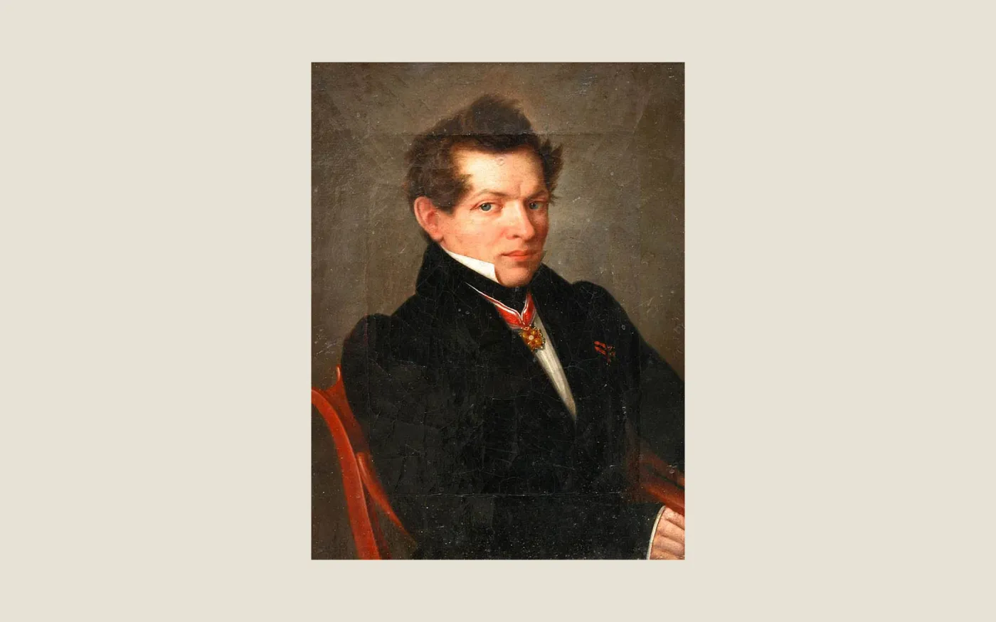
In February 1826, at Kazan University, a lecturer brought a work on the foundations of geometry before the department. Nikolai Lobachevsky was moving beyond something students rarely questioned: that the geometry drawn on paper was the only possible geometry. The manuscript from that occasion has not survived, so we do not know exactly how the work was presented.[1]
Do a triangle’s angles always add up to 180°? Only if we mean a triangle in the Euclidean plane. In Lobachevsky’s non-Euclidean geometry, every nondegenerate triangle with three vertices inside the plane has an angle sum below 180°. This is not a faulty protractor or a missing angle. The geometric assumptions have changed.[8]
You can tear the three corners off a paper triangle and arrange them into a straight angle. That works on a flat sheet. But why should the result apply to every possible space? Starting with this familiar question, we will follow Lobachevsky’s construction of another geometry, calculate a specific triangle, and trace the connection through Riemann to Einstein’s account of gravity.
This is part 3 of a three-part series on the parallel postulate and non-Euclidean geometry. Part 1 covers Euclid and the axiomatic method; part 2 follows János Bolyai and whether there is only one parallel.
What do triangle angles have to do with parallel lines?
Draw triangle ABC on paper. Through A, draw a line parallel to BC. Using alternate interior angles, move the angles at B and C to either side of angle A. The three angles sit next to one another along a straight line, so they add up to 180°.
One step in that familiar proof is not free: drawing the parallel and using its associated angle properties. In the usual foundations of geometry, the statement that every triangle has an angle sum of 180° is tied to the parallel postulate. It is not an independent fact we may carry unchanged into any set of assumptions.[4]
Cutting the corners off a paper triangle and fitting them together does not escape this issue. The flat sheet is already a Euclidean case. An experiment on paper checks what happens in that case, not whether every geometry must resemble the sheet.
Drawing two parallel lines gives another familiar result: their perpendicular separation is constant. You use that property to check a plank’s width. Changing the parallel assumption means reexamining both the triangle angle sum and equal separation, rather than keeping them simply because they are familiar.
The familiar assumption is: in the same plane, through a point outside a straight line, there is one and only one straight line parallel to the given line. The article on Euclid and the axiomatic method explains why this is an equivalent formulation, not the original wording of Euclid’s fifth postulate.
For Lobachevsky, the question went beyond drawing an additional line. If those other lines are admitted, how should angles, triangles, and distances work? A different set of rules must answer ordinary questions too, such as which route is shortest from where you stand to a wall.
At Kazan, more than a counterexample was needed
Lobachevsky spent much of their career at Kazan University. Teaching went alongside administrative work; in 1827, they became rector. The geometry developed amid those responsibilities, not in a separate contest to find the shortest answer to the parallel postulate.[1]
The presentation took place on February 11, 1826, under the Julian calendar then used in Russia, or February 23 under the Gregorian calendar. The two dates sometimes found in biographies refer to the same event. Since the manuscript is lost, we should not invent dialogue or audience reactions.[1][2]
The work began appearing in print in 1829 and continued into 1830 in the Kazan Messenger. This is a publication milestone, not proof that everything in the printed version had already appeared unchanged in the presentation three years earlier.[1][2]
Lobachevsky published the new geometry independently of János Bolyai. In the story of Bolyai’s 1823 letter, the focus was the change of question: stop trying to force the fifth postulate to become a theorem. At Kazan, we follow the next task: turn a different assumption into a system specific enough for calculation and publication.
A triangle whose angles add up to about 146°
To see what changes, place A, B, and C at the same three coordinates. On the left, connect them with Euclidean straight segments. On the right, connect them using hyperbolic straight lines, represented by arcs perpendicular to the boundary. The same vertex coordinates do not give the same triangle, because the rules defining its sides differ.
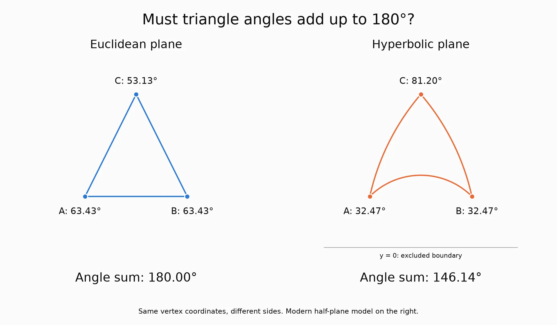
| Geometry of this example | Angle A | Angle B | Angle C | Sum |
|---|---|---|---|---|
| Euclidean | 63.434949° | 63.434949° | 53.130102° | 180° |
| Hyperbolic | 32.471192° | 32.471192° | 81.202589° | 146.144974° |
Each side on the right is a segment of a geodesic: a path that is straight within that geometry and locally shortest. Just as a Hanoi–Paris flight route looks curved on a flat map while the aircraft does not circle around, the curve in the picture comes from the drawing. So do not measure the angles of straight chords and assign them to the right-hand triangle. The angle between curved sides is the angle between their tangent directions at the vertex. Think of roads meeting: the turn depends on their directions at the junction, not a straight segment between distant places. This model preserves angles, so tangent measurements give the hyperbolic angles.[5]
The amount missing from 180° is the angular defect. If 180° is the expected budget, this triangle falls short by about 33.855026°. This is not measurement error. In a hyperbolic plane of fixed curvature, the defect is proportional to the triangle’s area.[8]
Not every triangle in this geometry has a sum of 146°. That number belongs to our example. Another triangle can be closer to 180° or fall further short. When a triangle is small compared with the curvature scale, its geometry approaches the flat case. A non-Euclidean system can therefore agree closely with everyday intuition on small scales.[4]
“Infinitely many” or “two” parallel lines?
This is where language can make two articles in the same series appear contradictory.
In the broad school-level usage, parallel lines are coplanar lines that do not intersect. In the hyperbolic plane, the non-Euclidean geometry considered here, infinitely many lines through an external point do not meet a given line.
But in the 1840 work, Lobachevsky reserved the word “parallel” for limiting parallels. Imagine standing at P and rotating a ray toward a line g. A range of directions leads to an intersection. Beyond a boundary direction, the ray no longer meets g. There are two boundaries, corresponding to the two directions along g.[3]
It is rather like rotating a flashlight to locate the edge of the region its beam reaches: the boundary direction matters. Here, however, there is no obstruction or finite edge of a wall. The boundary separates directions that intersect an indefinitely extended line from directions that do not.
Thus “infinitely many non-intersecting lines” and “two limiting parallels” count different sets. The remaining non-intersecting lines do not belong to this boundary pair; they have a common perpendicular with g. The pair in the following illustration consists of limiting parallels.
Two lines never meet, but their separation changes
We will use a modern representation, the Poincaré half-plane model. Think of a map whose scale changes with position: locations on the sheet do not directly give distances in the geometry it represents. This is not a drawing Lobachevsky made in 1826.[5]
The domain consists only of the region above the horizontal axis, where y is greater than 0. The boundary y = 0 is not part of this plane. Its straight lines are represented by vertical lines or semicircles perpendicular to the boundary.[5]
Choose two vertical lines, g and h, with horizontal coordinates 0 and 1. They do not meet inside the domain. On h, choose P₁, P₂, and P₃, ordered from bottom to top. For each point, find the shortest route to g.
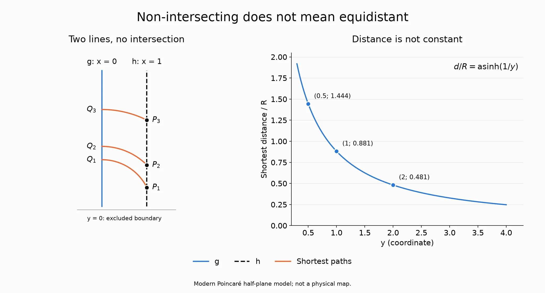
On paper, the horizontal gap between the lines is always 1. Measuring under the hyperbolic rule gives the following results. These are my calculations within the model, not measurements of physical space:
| Point on h | Coordinate y | Shortest distance to g, divided by R |
|---|---|---|
| P₁ | 0.5 | 1.443635 |
| P₂ | 1 | 0.881374 |
| P₃ | 2 | 0.481212 |
Moving upward along h brings you closer to g under this measurement. Yet there is no finite point where the lines meet. The distance can become arbitrarily small without becoming 0 at any point on h. Think of a sequence of positive numbers decreasing toward 0: approaching 0 does not require any term to equal 0.
The orange arcs are the easiest part to misread. They are perpendicular to g at their endpoints, but not necessarily perpendicular to h where they begin. We are measuring the distance from each point to a line, not looking for a common perpendicular between the two lines.
Why did publication not bring acceptance?
The reception of Lobachevsky’s work involved specific obstacles. Ostrogradsky assessed it negatively when it was submitted to the academy in St Petersburg. In 1834, Syn otechestva published a mocking attack. These events do not establish that every colleague responded in the same way.[1][2]
Lobachevsky kept seeking readers beyond Kazan. In 1837, Géométrie imaginaire appeared in French in Crelle’s Journal. In 1840, the German book Geometrische Untersuchungen zur Theorie der Parallellinien appeared in Berlin.[1][4]
The name “imaginary geometry” can mislead. It did not mean that the author could imagine any conclusion they pleased. The work still had to prove the consequences of its assumptions. A game may have unfamiliar rules without allowing arbitrary moves.
The 1840 book attracted Gauss’s attention. On Gauss’s recommendation, Lobachevsky was elected to the Göttingen scientific society in 1842. The story that “no one recognized the work during Lobachevsky’s lifetime” therefore goes too far.[1][2]
But this should not become a story of public advocacy either. Gauss did not publicly campaign for the theory, and there was no personal correspondence with Lobachevsky. MacTutor also corrects the claim that Gauss learned Russian solely to read this work: the language study had begun earlier.[1]
The difficulty was not merely finding someone willing to listen. The new geometry also needed a way for readers to place it within mathematics they already understood. Beltrami’s models in 1868, after Lobachevsky had passed away, were an important step in that direction.[4]
What does a model let us trust?
A mathematical model, in this setting, gives concrete meanings to objects and checks the rules they satisfy. As when squares and coordinates on a board implement a game, we must specify what counts as a point, a line, and a length.
If hyperbolic geometry can be constructed within Euclidean mathematics, a contradiction derived from hyperbolic rules would also produce a contradiction in the framework used to construct the model. This is relative consistency: a conditional assurance, rather like checking a translation through the language used to interpret it. It is not an absolute proof that all mathematics is free of contradiction.
From Lobachevsky to Riemann: more than two geometries
Triangles adding up to 180° or less than 180° are not the whole story. On a sphere, construct a triangle with three right angles. Travel from the North Pole to the equator along a meridian, follow a quarter of the equator, then return along another meridian. All three sides follow great circles, intrinsically straight paths on the sphere. The angles add up to 270°.[9]
No sphere is hidden inside the hyperbolic picture above. The cases differ: a sphere has positive curvature, while Lobachevsky’s plane has constant negative curvature. The Euclidean plane has zero curvature. Curvature is something an observer inside the geometry can detect through measurements, such as a triangle’s deviation from 180°. It is not merely how a sheet appears to bend upward or downward when viewed from outside.[9]
In 1854, Bernhard Riemann presented a broader approach. Instead of choosing only among a few models, one could study spaces with length-measurement rules defined at each location. The lecture was published in 1868. Curvature need not be the same everywhere, and spaces need not be limited to two dimensions.[4]
Think of a map with local measurement instructions in each region. To measure a journey, combine small segments according to the local instructions. This comparison explains the measurement rule’s role; it does not mean that changing a map’s scale creates every kind of curvature. What matters is the space’s own measuring structure, not its presentation.
Lobachevsky and Bolyai showed that Euclidean geometry was not the only logical possibility. Riemann broadened the language for studying geometric structures. This became part of the mathematical background to a later physical question: if geometry need not be settled in advance, could the distribution of matter be related to the geometry of the world?
How does relativity use this idea?
Release an object inside a freely falling cabin and it floats relative to the cabin. Astronauts aboard a space station are also in continuous free fall, not beyond the reach of gravity. This leads to an important idea in general relativity: over a sufficiently small region and brief period, a freely falling frame can remove the effects of a uniform gravitational field locally.[9]
Across a larger region, however, something remains that a change of viewpoint cannot erase. Objects falling at different positions can change their separation because the gravitational field is not uniform. This is a tidal effect: differences in gravity make different parts of an object move differently. Think of two people following meridians: each walks straight on the sphere, yet their separation changes.[9]
Einstein describes gravity through the geometry of spacetime. An event needs both a location and a time, just as meeting at a café requires an address and an appointment time. Spacetime therefore has three spatial dimensions and one temporal dimension. Our two-coordinate triangle picture illustrates a simpler idea, not this entire structure.
A test object subject only to gravity follows a spacetime geodesic. Its spatial track can look curved on a map, while geometrically it follows an intrinsically straightest path. Light also follows geodesics, of the type appropriate to light. This connects geometry to falling objects and deflected light, rather than merely to drawing triangles.[9]
Matter and energy are related to curvature through Einstein’s field equations. Think of two sides of a comparison: one describes geometry, the other the sources of matter and energy. This is a physical theory requiring observational tests, not an automatic consequence of dropping the parallel postulate. Lobachevsky did not derive gravitational field equations from triangles below 180°.[9]
Two limits are essential. First, general relativity does not say that spacetime is always a hyperbolic space of constant negative curvature. It uses a Lorentzian structure: its measurement rule distinguishes temporal from spatial directions fundamentally. Figure 1 cannot determine the angle sum of a “spacetime triangle.” Even special relativity’s flat spacetime is not four-dimensional Euclidean space.
Second, the timelike geodesic of a freely falling object is not simply a “shortest-length path” like an orange arc in Figure 2. The time recorded by a carried clock has its own role. A timelike geodesic makes this proper time stationary and, in a suitable local setting, maximal rather than minimal. The connection is that geometry determines what counts as straight and what is measured, not that every curved picture uses the same ruler.
So the connection between non-Euclidean geometry and relativity is real, but it passes through several layers: Lobachevsky and Bolyai ended Euclid’s monopoly, Riemann built a general language, and Einstein used that language for a physical theory. Lobachevsky did not write Einstein’s theory in advance.
Was Euclid wrong, and must the universe be curved?
No. Euclidean geometry remains valid as a theory with its own assumptions. Another system does not invalidate it, just as the rules of Go do not turn a legal chess move into an illegal one.
Nor can either illustration establish that physical space has precisely Lobachevsky’s geometry. A mathematical model tells us what follows from a set of rules; which rules describe the world is a question for physical observation.
Finally, a “circular arc on screen” does not mean a traveler inside the geometry must keep turning. It is a geodesic drawn on a map. The flight-route comparison only separates a map from a path; a sphere is not the hyperbolic plane.
Where did the ruler change?
If you only want the story, the main point is already in place: a 180° angle sum and equidistant parallels are consequences of Euclidean geometry, not of every geometry. This section opens up the model’s ruler to check the numbers.
The measurement rule, called a metric, resembles a map legend stating how each small drawn segment translates into length. In the half-plane, it takes the form:
MathWorld gives the normalized form with R = 1; keeping R here makes the length scale visible.[5] The same small segment on paper has a shorter hyperbolic length at larger y. But we cannot take a horizontal segment of length 1, divide by y, and declare that the shortest distance. A horizontal line is not a geodesic of this model.
For P = (1, y), the nearest point on g is Q = (0, √(1 + y²)). The circular arc centered at (0, 0) through P and Q is a geodesic, perpendicular to g at Q. Write its radius as r and parameterize it by angle t: x = r cos t and y = r sin t along the arc. Here y in the parameterization changes along the path, whereas the y of P is the fixed starting coordinate.
Substituting into the measurement rule makes the length divided by R the integral of 1/sin t from the starting angle to π/2. The result is:
The function asinh is simply a compact way to write the logarithmic expression in the middle. Substituting y = 0.5, 1, and 2 gives the distance table beside Figure 2.
For constant curvature K = −1/R², the triangle area is S = R²[π − (α + β + γ)], with angles measured in radians. The term in brackets is the angular defect. In our example it is about 0.590882, giving area 0.590882R². This relates size to the departure from flat geometry. It is a formula for the hyperbolic plane, not an equation for arbitrary spacetime triangles.[8]
In the 1840 work, Lobachevsky developed another relationship: the angle of parallelism. It is the angle between the perpendicular direction from P toward g and a limiting parallel ray. Rather like adjusting a sighting direction when you change position, this angle depends on the distance from P to g.[3]
In modern notation, for perpendicular distance a, the formula is tan(Π(a)/2) = exp(−a/R). The original chooses a suitable length unit instead of retaining R in this form. The point is not to memorize an exponential function. Distance has entered a question about direction: in the new geometry, the limiting angle is not fixed at 90°.[3]
Calculate the angles of a non-Euclidean triangle
This NumPy and Matplotlib code generates Figure 1 and saves images/lobachevsky-kazan/tong-goc-tam-giac-en.png. It uses A = (−1, 1), B = (1, 1), C = (0, 3), with no random inputs. Each hyperbolic side is an arc perpendicular to y = 0; the angle comes from its tangent vectors, not from the straight chords.
from pathlib import Pathimport numpy as npimport matplotlibmatplotlib.use('Agg')import matplotlib.pyplot as plt
out = Path('images/lobachevsky-kazan')out.mkdir(parents=True, exist_ok=True)en = Truepoints = np.array([[-1., 1.], [1., 1.], [0., 3.]])
# Arcs perpendicular to y=0; return the tangent at p too.def side(p, q):    center = (q @ q - p @ p) / (2 * (q[0] - p[0]))    radius = np.linalg.norm(p - [center, 0])    angles = np.arctan2([p[1], q[1]], [p[0]-center, q[0]-center])    t = np.linspace(*angles, 180)    path = np.c_[center + radius*np.cos(t), radius*np.sin(t)]    tangent = np.array([-p[1], p[0]-center])    return path, tangent * np.sign(angles[1] - angles[0])
hyper, flat = [], []for i, p in enumerate(points):    q, r = points[(i+1) % 3], points[(i+2) % 3]    for values, u, v in ((hyper, side(p,q)[1], side(p,r)[1]),                          (flat, q-p, r-p)):        cosine = np.dot(u,v) / (np.linalg.norm(u)*np.linalg.norm(v))        values.append(np.degrees(np.arccos(np.clip(cosine,-1,1))))assert abs(sum(flat) - 180) < 1e-10assert 0 < sum(hyper) < 180plt.rcParams.update({'font.family':'DejaVu Sans','font.size':14,                     'text.color':'#0b0b0b'})fig, axes = plt.subplots(1,2,figsize=(12,7),facecolor='#fcfcfb')for k, (ax, values, color) in enumerate(zip(axes,[flat,hyper],['#2a78d6','#eb6834'])):    ax.set_facecolor('#fcfcfb')    for i,p in enumerate(points):        q=points[(i+1) % 3]        path = np.array([p,q]) if k == 0 else side(p,q)[0]        ax.plot(*path.T,color=color,lw=2)    for i,(p,value) in enumerate(zip(points,values)):        ax.plot(*p,'o',color=color,ms=8,mec='#fcfcfb',mew=1.5)        dx,dy = [(-.1,-.3),(.1,-.3),(0,.25)][i]        ax.text(p[0]+dx,p[1]+dy,f'{"ABC"[i]}: {value:.2f}°',                ha='center',va='center',color='#0b0b0b')    if k:        ax.axhline(0,color='#999999',lw=.8)        ax.text(0,-.2,'y = 0: excluded boundary' if en else 'y = 0: biên không thuộc mặt phẳng',                ha='center',fontsize=10)    ax.set(xlim=(-1.9,1.9),ylim=(-.5,3.7),aspect='equal')    ax.axis('off')    title = ('Euclidean plane' if en else 'Mặt phẳng Euclid') if k==0 else (             'Hyperbolic plane' if en else 'Mặt phẳng hyperbolic')    ax.set_title(title,fontsize=18,pad=16)    ax.text(.5,-.04,('Angle sum: ' if en else 'Tổng ba góc: ')+f'{sum(values):.2f}°',            transform=ax.transAxes,ha='center',fontsize=19)fig.suptitle('Must triangle angles add up to 180°?' if en else             'Tổng ba góc tam giác luôn bằng 180°?',fontsize=23,y=.96)fig.text(.5,.035,'Same vertex coordinates, different sides. Modern half-plane model on the right.' if en else         'Cùng tọa độ đỉnh, khác đường cạnh. Bên phải dùng mô hình nửa mặt phẳng hiện đại.',         ha='center',fontsize=11)fig.subplots_adjust(left=.04,right=.96,bottom=.16,top=.82,wspace=.25)fig.savefig(out/('tong-goc-tam-giac-en.png' if en else 'tong-goc-tam-giac.png'),dpi=160)plt.close(fig)print('Euclid:', ', '.join(f'{x:.6f}' for x in flat), 'sum =', f'{sum(flat):.6f}')print('Hyperbolic:', ', '.join(f'{x:.6f}' for x in hyper), 'sum =', f'{sum(hyper):.6f}')
Running the code gives 180.000000° for the Euclidean sum and 146.144974° for the hyperbolic sum, with individual angles listed beside Figure 1. Rounding the three displayed angles separately may change the last decimal of their sum.
This calculation checks one example, not every triangle. It illustrates the general theorem without replacing its proof. The helper handles the nonvertical sides used here; coinciding vertices or vertical sides require separate handling before changing the coordinates.
Return to the work sent from Kazan
We cannot put the 1826 manuscript on a desk and read its exact words. What we can follow is a sequence of publications, from the Russian article in Kazan to presentations in French and German. An idea needs to become a system that other people can check, not merely a story about finding an answer.
In the final years, after losing their sight, Lobachevsky still completed Pangeometry. The Russian version appeared in 1855 and the French version in 1856. The European Mathematical Society’s scholarly edition now places both originals alongside a translation.[1][6]
The three torn corners of a paper triangle still make a straight angle. Lobachevsky did not make that classroom experiment wrong. The work showed why a result about a flat sheet cannot decide every possible geometry. From there, asking which geometry describes the physical world became a question for theory and measurement, not a conclusion fixed by the paper in our hands.
Previous in the series: János Bolyai: Is there really only one parallel?. Start the series from the beginning: Euclid and the axiomatic method.
Free geometry illustrations for students and teachers: EyeViz.
Tài liệu tham khảo
- [1]J. J. O’Connor and E. F. Robertson. Nikolai Ivanovich Lobachevsky. MacTutor History of Mathematics, University of St Andrews.
- [2]B. A. Rosenfeld. Lobachevsky, Nikolai Ivanovich. Dictionary of Scientific Biography, hosted by MacTutor.
- [3]Nikolai Lobachevsky; translated by George Bruce Halsted. Geometrical Researches on the Theory of Parallels. Open Court, translation of the Berlin 1840 work, 1914.
- [4]J. J. O’Connor and E. F. Robertson. Non-Euclidean geometry. MacTutor History of Mathematics, University of St Andrews.
- [5]Eric W. Weisstein. Poincaré Half-Plane Model. MathWorld, Wolfram Research.
- [6]Nikolai I. Lobachevsky; translated and edited by Athanase Papadopoulos. Pangeometry. European Mathematical Society, 2010.
- [7]Lev Kryukov. Lobachevsky.jpg. Wikimedia Commons, public domain.
- [8]Eric W. Weisstein. Hyperbolic Triangle. MathWorld, Wolfram Research.
- [9]Markus Pössel. Gravity: from weightlessness to curvature. Einstein Online, Max Planck Institute for Gravitational Physics.